Unit Conversion#
The sdf_xarray package automatically extracts the units for each
coordinate/variable/constant from an SDF file and stores them as an xarray.Dataset
attribute called "units". Sometimes we want to convert our data from one format to
another, e.g. converting the grid coordinates from meters to microns, time from seconds
to femto-seconds or particle energy from Joules to electron-volts.
import sdf_xarray as sdfxr
import matplotlib.pyplot as plt

plt.rcParams.update({
    "axes.labelsize": 16,
    "xtick.labelsize": 14,
    "ytick.labelsize": 14,
    "axes.titlesize": 16,
    "figure.titlesize": 18,
})
Rescaling coordinates#
For simple scaling and unit relabelling of coordinates (e.g., converting meters to microns),
the most straightforward approach is to use the xarray.Dataset.epoch.rescale_coords dataset accessor.
This function scales the coordinate values by a given multiplier and updates the
"units" attribute in one step. If the multiplier is not specified then the conversion parameter is inferred from the units and converted automatically using pint (see Unit conversion with pint-xarray for details).
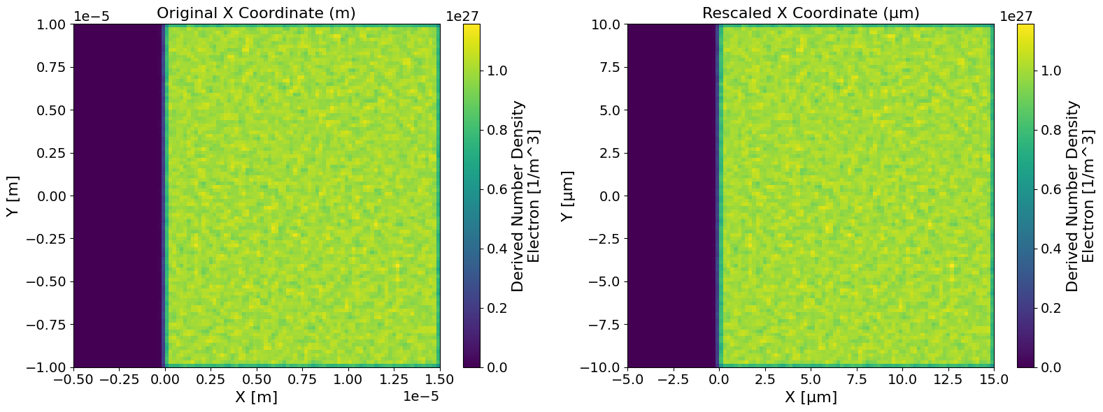
Rescaling grid coordinates#
We can use the xarray.Dataset.epoch.rescale_coords method to convert X, Y, and Z coordinates from meters
(m) to microns (µm) by applying a multiplier of 1e6.
fig, (ax1, ax2) = plt.subplots(1, 2, figsize=(16, 6))

ds = sdfxr.open_mfdataset("tutorial_dataset_2d/*.sdf")
ds_in_microns = ds.epoch.rescale_coords("µm", ["X_Grid_mid", "Y_Grid_mid"], 1e6)

ds["Derived_Number_Density_Electron"].isel(time=0).epoch.plot(ax=ax1)
ax1.set_title("Original X Coordinate (m)")

ds_in_microns["Derived_Number_Density_Electron"].isel(time=0).epoch.plot(ax=ax2)
ax2.set_title("Rescaled X Coordinate (µm)")

fig.tight_layout()
Rescaling time coordinate#
We can also use the xarray.Dataset.epoch.rescale_coords method to convert the time coordinate from
seconds (s) to femto-seconds (fs).
ds = sdfxr.open_mfdataset("tutorial_dataset_2d/*.sdf")
ds["time"]
<xarray.DataArray 'time' (time: 21)> Size: 168B
array([1.886923e-16, 1.018939e-14, 2.000139e-14, 3.019078e-14, 4.000278e-14,
       5.019216e-14, 6.000417e-14, 7.019355e-14, 8.000556e-14, 9.019494e-14,
       1.000069e-13, 1.101963e-13, 1.200083e-13, 1.301977e-13, 1.400097e-13,
       1.501991e-13, 1.600111e-13, 1.702005e-13, 1.800125e-13, 1.902019e-13,
       2.000139e-13])
Coordinates:
  * time     (time) float64 168B 1.887e-16 1.019e-14 2e-14 ... 1.902e-13 2e-13
Attributes:
    units:      s
    long_name:  Time
full_name: timeds = ds.epoch.rescale_coords("fs", "time")
ds["time"]
<xarray.DataArray 'time' (time: 21)> Size: 168B
array([1.886923e-01, 1.018939e+01, 2.000139e+01, 3.019078e+01, 4.000278e+01,
       5.019216e+01, 6.000417e+01, 7.019355e+01, 8.000556e+01, 9.019494e+01,
       1.000069e+02, 1.101963e+02, 1.200083e+02, 1.301977e+02, 1.400097e+02,
       1.501991e+02, 1.600111e+02, 1.702005e+02, 1.800125e+02, 1.902019e+02,
       2.000139e+02])
Coordinates:
  * time     (time) float64 168B 0.1887 10.19 20.0 30.19 ... 180.0 190.2 200.0
Attributes:
    long_name:  Time
    full_name:  time
units: fsUnit conversion with pint-xarray#
While this is sufficient for most use cases, we can enhance this functionality
using the pint library.
Pint allows us to specify the units of a given array and convert them
to another, which is incredibly handy. We can take this a step further,
however, and utilize the pint-xarray
library. This library allows us to infer units directly from an
xarray.Dataset.attrs while retaining all the information about the
xarray.Dataset. This works very similarly to taking a NumPy array and
multiplying it by a constant or another array, which returns a new array;
however, this library will also retain the unit logic (specifically the
"units" information).
Note
Unit conversion is not supported on coordinates in pint_xarray which is due to an
underlying issue with how xarray implements indexes.
Installation#
To install the pint libraries you can simply run the following optional
dependency pip command which will install both the pint and pint_xarray
libraries. Once installed the
xarray.Dataset.pint
accessor should become accessible. You can install these optional dependencies via pip:
pip install "sdf_xarray[pint]"
Quantifying DataArrays#
When using pint_xarray, the library attempts to infer units from the
"units" attribute on each xarray.DataArray. In the following example we will
extract the time-resolved total particle energy of electrons which is measured in
Joules and convert it to electron volts.
ds = sdfxr.open_mfdataset("tutorial_dataset_1d/*.sdf")
ds["Total_Particle_Energy_Electron"]
<xarray.DataArray 'Total_Particle_Energy_Electron' (time: 41)> Size: 328B
array([3.63855642e+06, 3.60115922e+06, 3.59514196e+06, 3.58946897e+06,
       3.25942169e+07, 1.98723930e+08, 4.39799138e+08, 1.18098588e+09,
       1.82893371e+09, 2.49245538e+09, 4.09498495e+09, 5.46823155e+09,
       6.86096603e+09, 8.12285559e+09, 9.01139219e+09, 9.87292528e+09,
       1.04479265e+10, 1.11933726e+10, 1.19621568e+10, 1.28297036e+10,
       1.29935776e+10, 1.25735119e+10, 1.15154093e+10, 1.15376467e+10,
       1.16272519e+10, 1.15725580e+10, 1.16607010e+10, 1.19066049e+10,
       1.16905460e+10, 1.15411511e+10, 1.13554034e+10, 1.14246777e+10,
       1.11812388e+10, 1.09841618e+10, 1.10835348e+10, 1.10507876e+10,
       1.10217255e+10, 1.10135640e+10, 1.09514926e+10, 1.08325276e+10,
       1.06959813e+10])
Coordinates:
  * time     (time) float64 328B 1.334e-16 5.07e-15 ... 1.951e-13 2.001e-13
Attributes:
    full_name:  Total Particle Energy/Electron
    long_name:  Total Particle Energy Electron
units: JOnce you call xarray.DataArray.pint.quantify the type is inferred the original
xarray.DataArray "units" attribute which is then removed and the data is
converted to a pint.Quantity.
Note
You can also specify the units yourself by passing it as a string
(e.g. "J") into the xarray.DataArray.pint.quantify function call.
total_particle_energy = ds["Total_Particle_Energy_Electron"].pint.quantify()
total_particle_energy
<xarray.DataArray 'Total_Particle_Energy_Electron' (time: 41)> Size: 328B
<Quantity([3.63855642e+06 3.60115922e+06 3.59514196e+06 3.58946897e+06
 3.25942169e+07 1.98723930e+08 4.39799138e+08 1.18098588e+09
 1.82893371e+09 2.49245538e+09 4.09498495e+09 5.46823155e+09
 6.86096603e+09 8.12285559e+09 9.01139219e+09 9.87292528e+09
 1.04479265e+10 1.11933726e+10 1.19621568e+10 1.28297036e+10
 1.29935776e+10 1.25735119e+10 1.15154093e+10 1.15376467e+10
 1.16272519e+10 1.15725580e+10 1.16607010e+10 1.19066049e+10
 1.16905460e+10 1.15411511e+10 1.13554034e+10 1.14246777e+10
 1.11812388e+10 1.09841618e+10 1.10835348e+10 1.10507876e+10
 1.10217255e+10 1.10135640e+10 1.09514926e+10 1.08325276e+10
 1.06959813e+10], 'joule')>
Coordinates:
  * time     (time) float64 328B [s] 1.334e-16 5.07e-15 ... 1.951e-13 2.001e-13
Indexes:
    time     PintIndex(PandasIndex, units={'time': 's'})
Attributes:
    full_name:  Total Particle Energy/Electron
long_name: Total Particle Energy ElectronNow that this dataset has been converted a pint.Quantity, we can check
it’s units and dimensionality
print(total_particle_energy.pint.units)
print(total_particle_energy.pint.dimensionality)
joule
[mass] * [length] ** 2 / [time] ** 2
Converting units#
We can now convert it to electron volts utilising the xarray.DataArray.pint.to
function
total_particle_energy_ev = total_particle_energy.pint.to("eV")
total_particle_energy_ev
<xarray.DataArray 'Total_Particle_Energy_Electron' (time: 41)> Size: 328B
<Quantity([2.27100829e+25 2.24766680e+25 2.24391112e+25 2.24037032e+25
 2.03437100e+26 1.24033721e+27 2.74501031e+27 7.37113409e+27
 1.14153064e+28 1.55566829e+28 2.55588857e+28 3.41300168e+28
 4.28227818e+28 5.06988769e+28 5.62446861e+28 6.16219527e+28
 6.52108281e+28 6.98635369e+28 7.46619105e+28 8.00767117e+28
 8.10995326e+28 7.84776886e+28 7.18735314e+28 7.20123265e+28
 7.25715981e+28 7.22302255e+28 7.27803708e+28 7.43151828e+28
 7.29666487e+28 7.20341992e+28 7.08748537e+28 7.13072294e+28
 6.97878032e+28 6.85577454e+28 6.91779828e+28 6.89735910e+28
 6.87921995e+28 6.87412596e+28 6.83538404e+28 6.76113193e+28
 6.67590644e+28], 'electron_volt')>
Coordinates:
  * time     (time) float64 328B [s] 1.334e-16 5.07e-15 ... 1.951e-13 2.001e-13
Indexes:
    time     PintIndex(PandasIndex, units={'time': 's'})
Attributes:
    full_name:  Total Particle Energy/Electron
long_name: Total Particle Energy ElectronUnit propagation#
Suppose instead of converting to "eV", we want to convert to "W"
(watts). To do this, we divide the total particle energy by time. However,
since coordinates in xarray.Dataset cannot be directly converted to
pint.Quantity, we must first extract the coordinate values manually
and create a new Pint quantity for time.
Once both arrays are quantified, Pint will automatically handle the unit propagation when we perform arithmetic operations like division.
Note
Pint does not automatically simplify "J/s" to "W", so we use
xarray.DataArray.pint.to to convert the unit string. Since
these units are the same it will not change the underlying data, only the
units. This is only a small formatting choice and is not required.
import pint

time_values = total_particle_energy.coords["time"].data
time = pint.Quantity(time_values, "s")
total_particle_energy_w = total_particle_energy / time # units: joule / second
total_particle_energy_w = total_particle_energy_w.pint.to("W") # units: watt
Dequantifying and restoring units#
Note
If this function is not called prior to plotting then the units will be
inferred from the pint.Quantity array which will return the long
name of the units. i.e. instead of returning "eV" it will return
"electron_volt".
The xarray.DataArray.pint.dequantify function converts the data from
pint.Quantity back to the original xarray.DataArray and adds
the "units" attribute back in. It also has an optional format parameter
that allows you to specify the formatting type of "units" attribute. We
have used the format="~P" option as it shortens the unit to its
“short pretty” format ("eV"). For more options, see the
Pint formatting documentation.
total_particle_energy_ev = total_particle_energy_ev.pint.dequantify(format="~P")
total_particle_energy_w = total_particle_energy_w.pint.dequantify(format="~P")
total_particle_energy_ev
<xarray.DataArray 'Total_Particle_Energy_Electron' (time: 41)> Size: 328B
array([2.27100829e+25, 2.24766680e+25, 2.24391112e+25, 2.24037032e+25,
       2.03437100e+26, 1.24033721e+27, 2.74501031e+27, 7.37113409e+27,
       1.14153064e+28, 1.55566829e+28, 2.55588857e+28, 3.41300168e+28,
       4.28227818e+28, 5.06988769e+28, 5.62446861e+28, 6.16219527e+28,
       6.52108281e+28, 6.98635369e+28, 7.46619105e+28, 8.00767117e+28,
       8.10995326e+28, 7.84776886e+28, 7.18735314e+28, 7.20123265e+28,
       7.25715981e+28, 7.22302255e+28, 7.27803708e+28, 7.43151828e+28,
       7.29666487e+28, 7.20341992e+28, 7.08748537e+28, 7.13072294e+28,
       6.97878032e+28, 6.85577454e+28, 6.91779828e+28, 6.89735910e+28,
       6.87921995e+28, 6.87412596e+28, 6.83538404e+28, 6.76113193e+28,
       6.67590644e+28])
Coordinates:
  * time     (time) float64 328B 1.334e-16 5.07e-15 ... 1.951e-13 2.001e-13
Attributes:
    full_name:  Total Particle Energy/Electron
    long_name:  Total Particle Energy Electron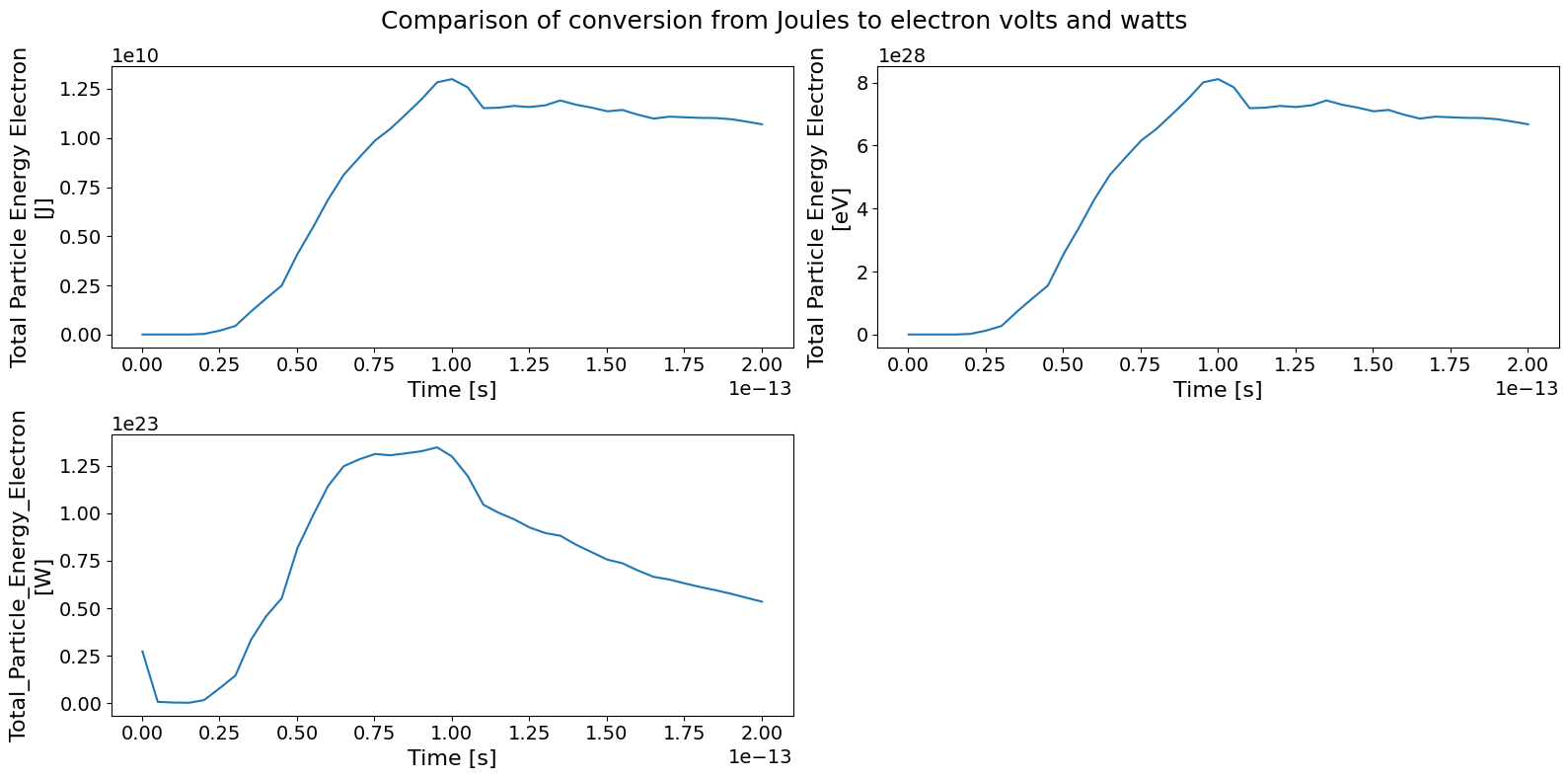
units: eVTo confirm the conversion has worked correctly, we can plot the original and
converted xarray.Dataset side by side:
fig, ((ax1, ax2), (ax3, ax4)) = plt.subplots(2, 2, figsize=(16,8))
ds["Total_Particle_Energy_Electron"].epoch.plot(ax=ax1)
total_particle_energy_ev.epoch.plot(ax=ax2)
total_particle_energy_w.epoch.plot(ax=ax3)
ax4.set_visible(False)
fig.suptitle("Comparison of conversion from Joules to electron volts and watts")
fig.tight_layout()