Histograms#
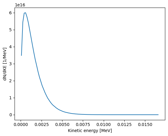
Plot Histogram Kinetic Energy Probes#
input deck:
datasets/5_1_probe/input.deckPython File:
histograms/plot_hist_ke_probe.py
from pathlib import Path

import matplotlib.pyplot as plt
import numpy as np

import sdf_xarray as sdfxr

# Constants
mass = 9.1093837e-31
c = 299792458
q0 = 1.60217663e-19

input_dir = Path("datasets/5_1_probe")
# Since we're loading particle and probes we need to specify their name
# from the input.deck
ds = sdfxr.open_mfdataset(
    input_dir, keep_particles=True, probe_names=["Electron_probe"]
)

px = ds["Electron_probe_Px"].values.flatten()
py = ds["Electron_probe_Py"].values.flatten()
pz = ds["Electron_probe_Pz"].values.flatten()
probe_weights_raw = ds["Electron_probe_weight"].values.flatten()

# Create a mask to remove NaNs
mask = ~np.isnan(probe_weights_raw)
probe_weights = probe_weights_raw[mask]
probe_px = px[mask]
probe_py = py[mask]
probe_pz = pz[mask]

probe_magnitude = probe_px**2 + probe_py**2 + probe_pz**2
ke_MeV = (np.sqrt(probe_magnitude * c**2 + mass**2 * c**4) - mass * c**2) / (1.0e6 * q0)

bin_edges = np.linspace(ke_MeV.min(), ke_MeV.max(), 101)
bin_N, _ = np.histogram(ke_MeV, bins=bin_edges, weights=probe_weights)
dKE = np.diff(bin_edges)
dN_dKE = bin_N / dKE
bin_centres = 0.5 * (bin_edges[:-1] + bin_edges[1:])

plt.plot(bin_centres, dN_dKE)
plt.xlabel("Kinetic energy [MeV]")
plt.ylabel("dN/dKE [1/MeV]")

plt.savefig(input_dir / "ke_spectrum.png", dpi=300)
np.savetxt(input_dir / "ke_spectrum_vals.txt", ke_MeV)
np.savetxt(input_dir / "ke_spectrum_ke.txt", bin_centres)
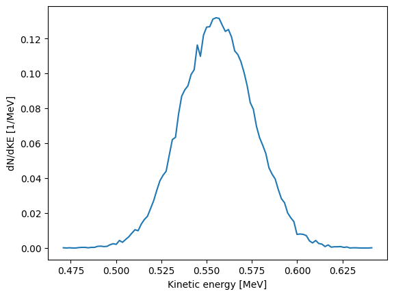
Plot Histogram Kinetic Energy#
input deck:
datasets/4_3_basic_target/input.deckPython File:
histograms/plot_hist_ke.py
from pathlib import Path

import matplotlib.pyplot as plt
import numpy as np

import sdf_xarray as sdfxr

# Constants
mass = 9.1093837e-31
c = 299792458
q0 = 1.60217663e-19

input_dir = Path("datasets/4_3_basic_target")
ds = sdfxr.open_dataset(input_dir / "0000.sdf", keep_particles=True)
particles_magnitude = (
    ds["Particles_Px_Electron"] ** 2
    + ds["Particles_Py_Electron"] ** 2
    + ds["Particles_Pz_Electron"] ** 2
)
ke_MeV = (np.sqrt(particles_magnitude * c**2 + mass**2 * c**4) - mass * c**2) / (
    1.0e6 * q0
)

bin_edges = np.linspace(ke_MeV.min().values, ke_MeV.max().values, 101)
bin_N, _ = np.histogram(
    ke_MeV.values, bins=bin_edges, weights=ds["Particles_Weight_Electron"]
)
dKE = np.diff(bin_edges)
dN_dKE = bin_N / dKE
bin_centres = 0.5 * (bin_edges[:-1] + bin_edges[1:])

plt.plot(bin_centres, dN_dKE)
plt.xlabel("Kinetic energy [MeV]")
plt.ylabel("dN/dKE [1/MeV]")

plt.savefig(input_dir / "ke_spectrum.png", dpi=300)
np.savetxt(input_dir / "ke_spectrum_vals.txt", ke_MeV.values)
np.savetxt(input_dir / "ke_spectrum_ke.txt", bin_centres)
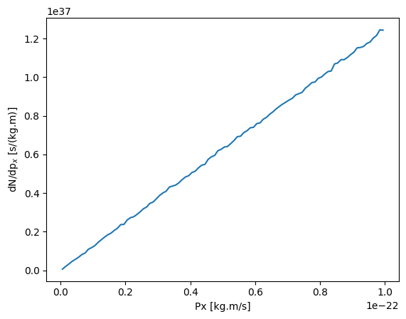
Plot Histogram Electron Momentum#
input deck:
datasets/4_4_momentum_distribution/input.deckPython File:
histograms/plot_hist_px.py
from pathlib import Path

import matplotlib.pyplot as plt
import numpy as np

import sdf_xarray as sdfxr

input_dir = Path("datasets/4_4_momentum_distribution")
ds = sdfxr.open_dataset(input_dir / "0000.sdf", keep_particles=True)
px = ds["Particles_Px_Electron_user"].values

bin_edges = np.linspace(px.min(), px.max(), 101)
bin_N, _ = np.histogram(
    px, bins=bin_edges, weights=ds["Particles_Weight_Electron_user"]
)
dpx = np.diff(bin_edges)
dN_dpx = bin_N / dpx
bin_centres = 0.5 * (bin_edges[:-1] + bin_edges[1:])

plt.plot(bin_centres, dN_dpx)
plt.xlabel("Px [kg.m/s]")
plt.ylabel("dN/dp$_x$ [s/(kg.m)]")

plt.savefig(input_dir / "px_spectrum.png", dpi=300)
np.savetxt(input_dir / "px_spectrum_vals.txt", dN_dpx)
np.savetxt(input_dir / "ke_spectrum_px.txt", bin_centres)