Animations

Animations#

Note

Unfortunately, these animations are not interactive like the rest of the documentation as building them on readthedocs takes too long so we display the GIFs from the datasets instead.

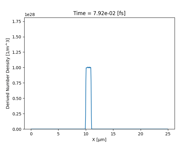
Animate Density 1D#

input deck: datasets/1_1_drifting_bunch/input.deck
Python File: animating/animate_1D_density.py

from pathlib import Path

import sdf_xarray as sdfxr

input_dir = Path("datasets/1_1_drifting_bunch")
ds = sdfxr.open_mfdataset(input_dir)

# Convert the time to femtoseconds
ds = ds.epoch.rescale_coords(1e15, "fs", "time")
# Convert the x and y coords to microns
ds = ds.epoch.rescale_coords(1e6, "µm", ["X_Grid_mid"])

anim = ds["Derived_Number_Density"].epoch.animate()

# Visualise it in a Jupyter notebook
anim.show()

# Or save the animation
# anim.save(input_dir / "number_density.gif", fps=5)

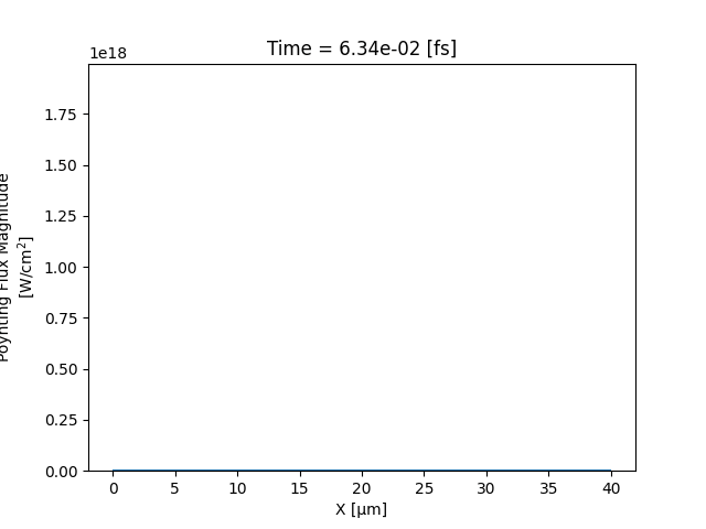
datasets/1_1_drifting_bunch/number_density.gif

Animate Poynting Flux 1D#

input deck: datasets/3_3_Gaussian_1d_laser/input.deck
Python File: animating/animate_1D_poynting_flux.py

from pathlib import Path

import numpy as np

import sdf_xarray as sdfxr

input_dir = Path("datasets/3_3_Gaussian_1d_laser")
ds = sdfxr.open_mfdataset(input_dir)

# Convert the time to femtoseconds
ds = ds.epoch.rescale_coords(1e15, "fs", "time")
# Convert the x and y coords to microns
ds = ds.epoch.rescale_coords(1e6, "µm", ["X_Grid_mid"])

# Calculate Poynting flux magnitude
flux_magnitude = np.sqrt(
    ds["Derived_Poynting_Flux_x"] ** 2
    + ds["Derived_Poynting_Flux_y"] ** 2
    + ds["Derived_Poynting_Flux_z"] ** 2
)

# convert to W/cm^2
I_Wcm2 = flux_magnitude * 1e-4
I_Wcm2.attrs["long_name"] = "Poynting Flux Magnitude"
I_Wcm2.attrs["units"] = "W/cm$^2$"

anim = I_Wcm2.epoch.animate()

# Visualise it in a Jupyter notebook
anim.show()

# Or save the animation
# anim.save(input_dir / "laser.gif", fps=10)

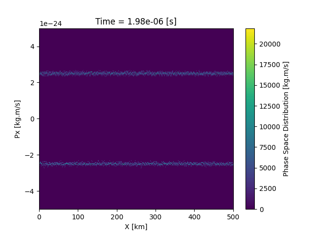
datasets/3_3_Gaussian_1d_laser/laser.gif

Animate Distribution Function Multi-Species 2D#

input deck: datasets/2_1_two_stream_instability/input.deck
Python File: animating/animate_2D_dist_fn_multispecies.py
Python File (alternative): animating/animate_2D_dist_fn_multispecies_alternative.py

from pathlib import Path

import sdf_xarray as sdfxr

input_dir = Path("datasets/2_1_two_stream_instability")
ds = sdfxr.open_mfdataset(
    input_dir, data_vars=["dist_fn_x_px_Left", "dist_fn_x_px_Right"]
)

# Rescale coords to account for kilometers
ds = ds.epoch.rescale_coords(1e-3, "km", ["X_x_px_Left"])

# Sum phase-space of species "Left" and "Right" in "x_px" distribution function
# NOTE: We only use the values from the right distribution function as if we inherit
# the coords we from the right we end up with 4 coords instead of 2
total_phase_space = ds["dist_fn_x_px_Left"] + ds["dist_fn_x_px_Right"].values
total_phase_space.attrs["long_name"] = "Phase Space Distribution"
total_phase_space.attrs["units"] = "kg.m/s"

anim = total_phase_space.epoch.animate()
# Visualise it in a Jupyter notebook
anim.show()

# Or save the animation
# anim.save(input_dir / "phase_space.gif")

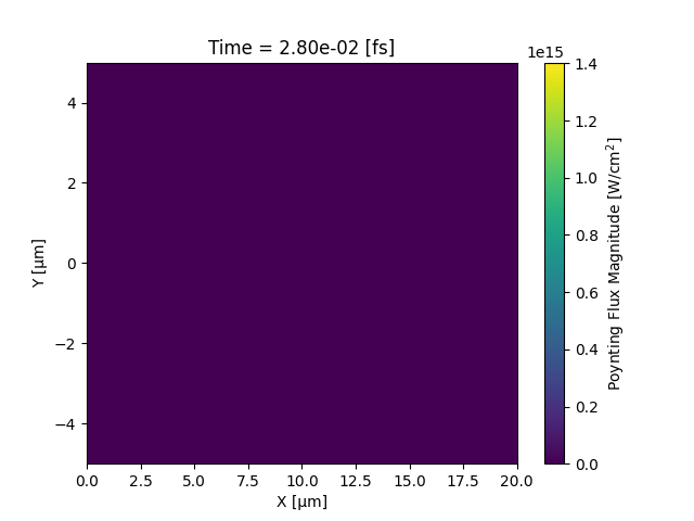
datasets/2_1_two_stream_instability/phase_space.gif

Animate Poynting Flux 2D#

input deck: datasets/3_5_Gaussian_beam/input.deck
Python File: animating/animate_2D_poynting_flux.py

from pathlib import Path

import numpy as np

import sdf_xarray as sdfxr

input_dir = Path("datasets/3_5_Gaussian_beam")
ds = sdfxr.open_mfdataset(input_dir)

# Convert the time to femtoseconds
ds = ds.epoch.rescale_coords(1e15, "fs", "time")
# Convert the x and y coords to microns
ds = ds.epoch.rescale_coords(1e6, "µm", ["X_Grid_mid", "Y_Grid_mid"])

# Calculate Poynting flux magnitude
flux_magnitude = np.sqrt(
    ds["Derived_Poynting_Flux_x"] ** 2
    + ds["Derived_Poynting_Flux_y"] ** 2
    + ds["Derived_Poynting_Flux_z"] ** 2
)

# convert to W/cm^2
I_Wcm2 = flux_magnitude * 1e-4
I_Wcm2.attrs["long_name"] = "Poynting Flux Magnitude"
I_Wcm2.attrs["units"] = "W/cm$^2$"

anim = I_Wcm2.epoch.animate()

# Visualise it in a Jupyter notebook
anim.show()

# Or save the animation
# anim.save(input_dir / "laser.gif", fps=10)

datasets/3_5_Gaussian_beam/laser.gif