Exploring and Manipulating Data#
When loading in either a single dataset or a group of datasets you can access the following methods to explore the dataset:
ds.variablesto list variables. (e.g. Electric Field, Magnetic Field, Particle Count)ds.coordsfor accessing coordinates/dimensions. (e.g. x-axis, y-axis, time)ds.attrsfor metadata attached to the dataset. (e.g. filename, step, time)
It is important to note here that xarray lazily loads the data
meaning that it only explicitly loads the results your currently
looking at when you call .values
import sdf_xarray as sdfxr
import matplotlib.pyplot as plt

ds = sdfxr.open_mfdataset("tutorial_dataset_1d/*.sdf")

ds["Electric_Field_Ex"]
<xarray.DataArray 'Electric_Field_Ex' (time: 41, X_Grid_mid: 200)> Size: 66kB
dask.array<concatenate, shape=(41, 200), dtype=float64, chunksize=(1, 200), chunktype=numpy.ndarray>
Coordinates:
  * time        (time) float64 328B 1.334e-16 5.07e-15 ... 1.951e-13 2.001e-13
  * X_Grid_mid  (X_Grid_mid) float64 2kB -4.95e-06 -4.85e-06 ... 1.495e-05
Attributes:
    units:       V/m
    point_data:  False
    full_name:   Electric Field/Ex
long_name: Electric Field $E_x$Visualisation#
sdf-xarray has built-in plotting and animation functionality, more details can
be found on Plotting and Animations.
Dimension slicing#
When loading a multi-file dataset using sdf_xarray.open_mfdataset, a
time dimension is automatically added to the resulting xarray.Dataset.
This dimension represents all the recorded simulation steps and allows
for easy indexing. To quickly determine the number of time steps available,
you can check the size of the time dimension.
ds = sdfxr.open_mfdataset("tutorial_dataset_1d/*.sdf")
# This corresponds to the number of individual SDF files loaded
print(f"There are a total of {ds['time'].size} time steps")

# You can look up the actual simulation time for any given index
sim_time = ds['time'].values[20]
print(f"The time at the 20th simulation step is {sim_time:.2e} s")
There are a total of 41 time steps
The time at the 20th simulation step is 1.00e-13 s
You can select and extract a single simulation snapshot using the integer
index of the time step with the xarray.Dataset.isel function. This can be
done by passing the index to the time parameter (e.g., time=0 for
the first snapshot).
ds["Electric_Field_Ex"].isel(time=20)
<xarray.DataArray 'Electric_Field_Ex' (X_Grid_mid: 200)> Size: 2kB
dask.array<getitem, shape=(200,), dtype=float64, chunksize=(200,), chunktype=numpy.ndarray>
Coordinates:
  * X_Grid_mid  (X_Grid_mid) float64 2kB -4.95e-06 -4.85e-06 ... 1.495e-05
    time        float64 8B 1.001e-13
Attributes:
    units:       V/m
    point_data:  False
    full_name:   Electric Field/Ex
long_name: Electric Field $E_x$We can also use the xarray.Dataset.sel function if you wish to pass a
value instead of an index.
Tip
If you know roughly what time you wish to select but not the exact value
you can use the parameter method="nearest".
ds["Electric_Field_Ex"].sel(time=sim_time)
<xarray.DataArray 'Electric_Field_Ex' (X_Grid_mid: 200)> Size: 2kB
dask.array<getitem, shape=(200,), dtype=float64, chunksize=(200,), chunktype=numpy.ndarray>
Coordinates:
  * X_Grid_mid  (X_Grid_mid) float64 2kB -4.95e-06 -4.85e-06 ... 1.495e-05
    time        float64 8B 1.001e-13
Attributes:
    units:       V/m
    point_data:  False
    full_name:   Electric Field/Ex
long_name: Electric Field $E_x$Manipulating data#
These datasets can also be easily manipulated the same way as you
would with numpy arrays.
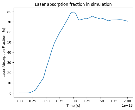
ds["Laser_Absorption_Fraction_in_Simulation"] = (
   (ds["Total_Particle_Energy_in_Simulation"] - ds["Total_Particle_Energy_in_Simulation"][0])
   / ds["Absorption_Total_Laser_Energy_Injected"]
) * 100

# We can also manipulate the units and other attributes
ds["Laser_Absorption_Fraction_in_Simulation"].attrs["units"] = "%"
ds["Laser_Absorption_Fraction_in_Simulation"].attrs["long_name"] = "Laser Absorption Fraction"

ds["Laser_Absorption_Fraction_in_Simulation"].epoch.plot()
plt.title("Laser absorption fraction in simulation")
plt.show()
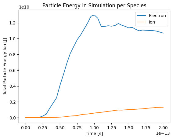
You can also call the xarray.DataArray.epoch.plot function on several variables with
labels by delaying the call to plt.show().
ds["Total_Particle_Energy_Electron"].epoch.plot(label="Electron")
ds["Total_Particle_Energy_Ion"].epoch.plot(label="Ion")
plt.title("Particle Energy in Simulation per Species")
plt.legend()
plt.show()
print(f"Total laser energy injected: {ds["Absorption_Total_Laser_Energy_Injected"][-1].values:.1e} J")
print(f"Total particle energy absorbed: {ds["Total_Particle_Energy_in_Simulation"][-1].values:.1e} J")
print(f"The laser absorption fraction: {ds["Laser_Absorption_Fraction_in_Simulation"][-1].values:.1f} %")
Total laser energy injected: 1.7e+10 J
Total particle energy absorbed: 1.2e+10 J
The laser absorption fraction: 70.6 %
Limit#
The .epoch accessor has the ability to “limit” data arrays. This is a helper
function which applies xarray.DataArray.where to the upper and lower bounds
of each dimension. You can use None to preserve the existing limit.
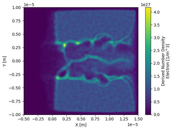
ds = sdfxr.open_dataset("tutorial_dataset_2d/0020.sdf")
da = ds["Derived_Number_Density_Electron"]
da.epoch.plot()
print(f"Orignal shape: {da.shape}")
plt.show()
Orignal shape: (100, 100)
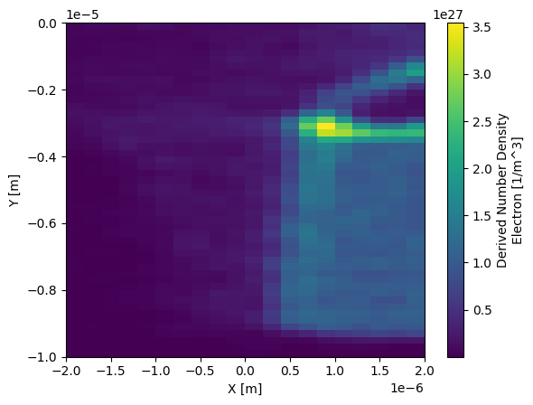
da_limit = da.epoch.limit(((-2e-6, 2e-6), (None, 0)))
da_limit.epoch.plot()
print(f"New shape: {da_limit.shape}")
plt.show()
New shape: (20, 50)
Resize#
The data arrays can be interpolated with sdf_xarray.dataarray_accessor.EpochAccessor.resize
to either increase or decrease the resolution while mantaining the general structure.
Decreasing the size may be useful to download large data from HPCs to local machines
or ploting with Voxel plots. Be aware that the original
data will not be preserved.
ds = sdfxr.open_dataset("tutorial_dataset_2d/0020.sdf")
da = ds["Derived_Number_Density_Electron"]

da.epoch.plot()
print(f"Orignal shape: {da.shape}")
plt.show()
Orignal shape: (100, 100)
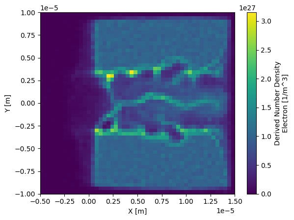
da_resized = da.epoch.resize((50, 50))
da_resized.epoch.plot()
print(f"New shape: {da_resized.shape}")
plt.show()
New shape: (50, 50)
Visualisation on HPC Machines#
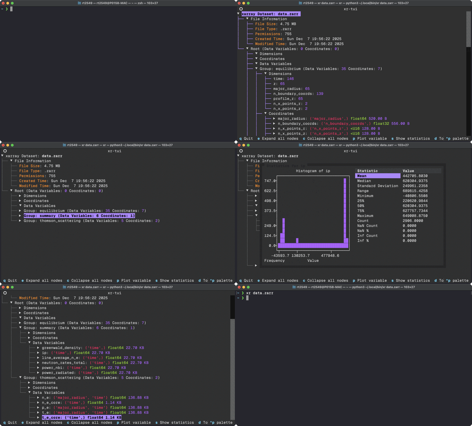
In many cases you will be running EPOCH simulations via a HPC cluster and your subsequent SDF files will probably be rather large and cumbersome to interact with via traditional Jupyter notebooks. In some cases your HPC may outright block the use of Jupyter notebooks entirely. To circumvent this issue you can use a Terminal User Interface (TUI) which renders the contents of SDF files directly in a Terminal and allows for you to do some simple data analysis and visualisation. To do this we shall leverage the xr-tui package which can be installed to either a venv or globally using:
pipx install xr-tui sdf-xarray
or if you are using uv
uv tool install xr-tui --with sdf-xarray
Once installed you can visualise SDF files by simply writing in the command line
xr path/to/simulation/0000.sdf
# OR
xr path/to/simulation/*.sdf
Below is an example gif of how this interfacing looks as seen on
xr-tui README.md: