Key Functionality#
In [1]: import xarray as xr

In [2]: import sdf_xarray as sdfxr

In [3]: import matplotlib.pyplot as plt

In [4]: from IPython.display import display, HTML
Loading SDF Files#
There are several ways to load SDF files:
To load a single file, use
xarray.open_dataset().To load multiple files, use
sdf_xarray.open_mfdataset()orxarray.open_mfdataset().To access the raw contents of a single SDF file, use
sdf_xarray.sdf_interface.SDFFile().
Note
When loading *.sdf files, variables related to boundaries, cpu and output file are excluded as they are problematic.
Loading a Single SDF File#
In [5]: xr.open_dataset("tutorial_dataset_1d/0010.sdf")
Out[5]:
<xarray.Dataset> Size: 246kB
Dimensions:                                       (X_Grid_mid: 1536,
                                                   X_Grid: 1537)
Coordinates:
  * X_Grid_mid                                    (X_Grid_mid) float64 12kB -...
  * X_Grid                                        (X_Grid) float64 12kB -1e-0...
Data variables: (12/27)
    Wall_time                                     float64 8B ...
    Electric_Field_Ex                             (X_Grid_mid) float64 12kB ...
    Electric_Field_Ey                             (X_Grid_mid) float64 12kB ...
    Electric_Field_Ez                             (X_Grid_mid) float64 12kB ...
    Magnetic_Field_Bx                             (X_Grid_mid) float64 12kB ...
    Magnetic_Field_By                             (X_Grid_mid) float64 12kB ...
    ...                                            ...
    Derived_Number_Density_Electron               (X_Grid_mid) float64 12kB ...
    Derived_Number_Density_Ion                    (X_Grid_mid) float64 12kB ...
    Derived_Number_Density_Photon                 (X_Grid_mid) float64 12kB ...
    Derived_Number_Density_Positron               (X_Grid_mid) float64 12kB ...
    Absorption_Total_Laser_Energy_Injected        float64 8B ...
    Absorption_Fraction_of_Laser_Energy_Absorbed  float64 8B ...
Attributes: (12/21)
    filename:         tutorial_dataset_1d/0010.sdf
    file_version:     1
    file_revision:    4
    code_name:        Epoch1d
    step:             960
    time:             5.003461427972353e-14
    ...               ...
    compile_machine:  login1.viking2.yor.alces.network
    compile_flags:    unknown
    defines:          50364608
    compile_date:     Fri Oct 11 15:12:01 2024
    run_date:         Fri Oct 25 11:34:55 2024
    io_date:          Fri Oct 25 11:35:51 2024
Loading a Single Raw SDF File#
In [6]: with sdfxr.SDFFile("tutorial_dataset_1d/0010.sdf") as sdf_file:
   ...:    print(sdf_file.variables)
   ...:
{'Wall-time': Constant(_id='elapsed_time', name='Wall-time', data=55.10663341684267, units=None), 'Electric Field/Ex': Variable(_id='ex', name='Electric Field/Ex', dtype=dtype('float64'), shape=(1536,), is_point_data=False, sdffile=<sdf_xarray.sdf_interface.SDFFile object at 0x7de1b6e1f940>, units='V/m', mult=1.0, grid='grid', grid_mid='grid_mid'), 'Electric Field/Ey': Variable(_id='ey', name='Electric Field/Ey', dtype=dtype('float64'), shape=(1536,), is_point_data=False, sdffile=<sdf_xarray.sdf_interface.SDFFile object at 0x7de1b6e1f940>, units='V/m', mult=1.0, grid='grid', grid_mid='grid_mid'), 'Electric Field/Ez': Variable(_id='ez', name='Electric Field/Ez', dtype=dtype('float64'), shape=(1536,), is_point_data=False, sdffile=<sdf_xarray.sdf_interface.SDFFile object at 0x7de1b6e1f940>, units='V/m', mult=1.0, grid='grid', grid_mid='grid_mid'), 'Magnetic Field/Bx': Variable(_id='bx', name='Magnetic Field/Bx', dtype=dtype('float64'), shape=(1536,), is_point_data=False, sdffile=<sdf_xarray.sdf_interface.SDFFile object at 0x7de1b6e1f940>, units='T', mult=1.0, grid='grid', grid_mid='grid_mid'), 'Magnetic Field/By': Variable(_id='by', name='Magnetic Field/By', dtype=dtype('float64'), shape=(1536,), is_point_data=False, sdffile=<sdf_xarray.sdf_interface.SDFFile object at 0x7de1b6e1f940>, units='T', mult=1.0, grid='grid', grid_mid='grid_mid'), 'Magnetic Field/Bz': Variable(_id='bz', name='Magnetic Field/Bz', dtype=dtype('float64'), shape=(1536,), is_point_data=False, sdffile=<sdf_xarray.sdf_interface.SDFFile object at 0x7de1b6e1f940>, units='T', mult=1.0, grid='grid', grid_mid='grid_mid'), 'Current/Jx': Variable(_id='jx', name='Current/Jx', dtype=dtype('float64'), shape=(1536,), is_point_data=False, sdffile=<sdf_xarray.sdf_interface.SDFFile object at 0x7de1b6e1f940>, units='A/m^2', mult=1.0, grid='grid', grid_mid='grid_mid'), 'Current/Jy': Variable(_id='jy', name='Current/Jy', dtype=dtype('float64'), shape=(1536,), is_point_data=False, sdffile=<sdf_xarray.sdf_interface.SDFFile object at 0x7de1b6e1f940>, units='A/m^2', mult=1.0, grid='grid', grid_mid='grid_mid'), 'Total Particle Energy/Electron': Constant(_id='total_particle_energy/Electron', name='Total Particle Energy/Electron', data=82091117810.61224, units='J'), 'Total Particle Energy/Ion': Constant(_id='total_particle_energy/Ion', name='Total Particle Energy/Ion', data=12465894316.948612, units='J'), 'Total Particle Energy/Photon': Constant(_id='total_particle_energy/Photon', name='Total Particle Energy/Photon', data=0.0, units='J'), 'Total Particle Energy/Positron': Constant(_id='total_particle_energy/Positron', name='Total Particle Energy/Positron', data=0.0, units='J'), 'Total Particle Energy in Simulation': Constant(_id='total_particle_energy', name='Total Particle Energy in Simulation', data=94557012127.56085, units='J'), 'Total Field Energy in Simulation': Constant(_id='total_field_energy', name='Total Field Energy in Simulation', data=3310272513246.5063, units='J'), 'Derived/Average_Particle_Energy': Variable(_id='ekbar', name='Derived/Average_Particle_Energy', dtype=dtype('float64'), shape=(1536,), is_point_data=False, sdffile=<sdf_xarray.sdf_interface.SDFFile object at 0x7de1b6e1f940>, units='J', mult=1.0, grid='grid', grid_mid='grid_mid'), 'Derived/Average_Particle_Energy/Electron': Variable(_id='ekbar/Electron', name='Derived/Average_Particle_Energy/Electron', dtype=dtype('float64'), shape=(1536,), is_point_data=False, sdffile=<sdf_xarray.sdf_interface.SDFFile object at 0x7de1b6e1f940>, units='J', mult=1.0, grid='grid', grid_mid='grid_mid'), 'Derived/Average_Particle_Energy/Ion': Variable(_id='ekbar/Ion', name='Derived/Average_Particle_Energy/Ion', dtype=dtype('float64'), shape=(1536,), is_point_data=False, sdffile=<sdf_xarray.sdf_interface.SDFFile object at 0x7de1b6e1f940>, units='J', mult=1.0, grid='grid', grid_mid='grid_mid'), 'Derived/Average_Particle_Energy/Photon': Variable(_id='ekbar/Photon', name='Derived/Average_Particle_Energy/Photon', dtype=dtype('float64'), shape=(1536,), is_point_data=False, sdffile=<sdf_xarray.sdf_interface.SDFFile object at 0x7de1b6e1f940>, units='J', mult=1.0, grid='grid', grid_mid='grid_mid'), 'Derived/Average_Particle_Energy/Positron': Variable(_id='ekbar/Positron', name='Derived/Average_Particle_Energy/Positron', dtype=dtype('float64'), shape=(1536,), is_point_data=False, sdffile=<sdf_xarray.sdf_interface.SDFFile object at 0x7de1b6e1f940>, units='J', mult=1.0, grid='grid', grid_mid='grid_mid'), 'Derived/Number_Density': Variable(_id='number_density', name='Derived/Number_Density', dtype=dtype('float64'), shape=(1536,), is_point_data=False, sdffile=<sdf_xarray.sdf_interface.SDFFile object at 0x7de1b6e1f940>, units='1/m^3', mult=1.0, grid='grid', grid_mid='grid_mid'), 'Derived/Number_Density/Electron': Variable(_id='number_density/Electron', name='Derived/Number_Density/Electron', dtype=dtype('float64'), shape=(1536,), is_point_data=False, sdffile=<sdf_xarray.sdf_interface.SDFFile object at 0x7de1b6e1f940>, units='1/m^3', mult=1.0, grid='grid', grid_mid='grid_mid'), 'Derived/Number_Density/Ion': Variable(_id='number_density/Ion', name='Derived/Number_Density/Ion', dtype=dtype('float64'), shape=(1536,), is_point_data=False, sdffile=<sdf_xarray.sdf_interface.SDFFile object at 0x7de1b6e1f940>, units='1/m^3', mult=1.0, grid='grid', grid_mid='grid_mid'), 'Derived/Number_Density/Photon': Variable(_id='number_density/Photon', name='Derived/Number_Density/Photon', dtype=dtype('float64'), shape=(1536,), is_point_data=False, sdffile=<sdf_xarray.sdf_interface.SDFFile object at 0x7de1b6e1f940>, units='1/m^3', mult=1.0, grid='grid', grid_mid='grid_mid'), 'Derived/Number_Density/Positron': Variable(_id='number_density/Positron', name='Derived/Number_Density/Positron', dtype=dtype('float64'), shape=(1536,), is_point_data=False, sdffile=<sdf_xarray.sdf_interface.SDFFile object at 0x7de1b6e1f940>, units='1/m^3', mult=1.0, grid='grid', grid_mid='grid_mid'), 'Absorption/Total Laser Energy Injected': Constant(_id='laser_enTotal', name='Absorption/Total Laser Energy Injected', data=3398487859758.498, units='J'), 'Absorption/Fraction of Laser Energy Absorbed': Constant(_id='abs_frac', name='Absorption/Fraction of Laser Energy Absorbed', data=1.0001282559889555, units='%'), 'CPUs/Original rank': Variable(_id='cpu_rank', name='CPUs/Original rank', dtype=dtype('int32'), shape=(96,), is_point_data=False, sdffile=<sdf_xarray.sdf_interface.SDFFile object at 0x7de1b6e1f940>, units='CPU', mult=None, grid='grid_cpu_rank', grid_mid='grid_cpu_rank_mid'), 'CPUs/Current rank': Variable(_id='cpus_current', name='CPUs/Current rank', dtype=dtype('int32'), shape=(0,), is_point_data=False, sdffile=<sdf_xarray.sdf_interface.SDFFile object at 0x7de1b6e1f940>, units='CPU', mult=None, grid='grid_cpus_current', grid_mid='grid_cpus_current_mid')}
Loading all SDF Files for a Simulation#
Multiple files can be loaded using one of two methods. The first of which
is by using the sdf_xarray.open_mfdataset()
In [7]: sdfxr.open_mfdataset("tutorial_dataset_1d/*.sdf")
Out[7]:
<xarray.Dataset> Size: 10MB
Dimensions:                                       (X_Grid: 1537,
                                                   X_Grid_mid: 1536, time: 41,
                                                   dim_laser_x_min_phase_0: 1,
                                                   dim_Random States_0: 384)
Coordinates:
  * X_Grid                                        (X_Grid) float64 12kB -1e-0...
  * X_Grid_mid                                    (X_Grid_mid) float64 12kB -...
  * time                                          (time) float64 328B 2.606e-...
Dimensions without coordinates: dim_laser_x_min_phase_0, dim_Random States_0
Data variables: (12/40)
    Wall_time                                     (time) float64 328B 0.4287 ...
    Electric_Field_Ex                             (time, X_Grid_mid) float64 504kB dask.array<chunksize=(1, 1536), meta=np.ndarray>
    Electric_Field_Ey                             (time, X_Grid_mid) float64 504kB dask.array<chunksize=(1, 1536), meta=np.ndarray>
    Electric_Field_Ez                             (time, X_Grid_mid) float64 504kB dask.array<chunksize=(1, 1536), meta=np.ndarray>
    Magnetic_Field_Bx                             (time, X_Grid_mid) float64 504kB dask.array<chunksize=(1, 1536), meta=np.ndarray>
    Magnetic_Field_By                             (time, X_Grid_mid) float64 504kB dask.array<chunksize=(1, 1536), meta=np.ndarray>
    ...                                            ...
    Particles_Particles_Per_Cell_Electron         (time) float64 328B nan ......
    Particles_Particles_Per_Cell_Ion              (time) float64 328B nan ......
    Particles_Particles_Per_Cell_Photon           (time) float64 328B nan ......
    Particles_Particles_Per_Cell_Positron         (time) float64 328B nan ......
    Random_States                                 (time, dim_Random States_0) float64 126kB dask.array<chunksize=(1, 384), meta=np.ndarray>
    Current_Jz                                    (time, X_Grid_mid) float64 504kB dask.array<chunksize=(1, 1536), meta=np.ndarray>
Attributes: (12/21)
    filename:         /home/docs/checkouts/readthedocs.org/user_builds/sdf-xa...
    file_version:     1
    file_revision:    4
    code_name:        Epoch1d
    step:             0
    time:             2.6059694937355635e-17
    ...               ...
    compile_machine:  login1.viking2.yor.alces.network
    compile_flags:    unknown
    defines:          50364608
    compile_date:     Fri Oct 11 15:12:01 2024
    run_date:         Fri Oct 25 11:34:55 2024
    io_date:          Fri Oct 25 11:34:57 2024
Alternatively files can be loaded using xarray.open_mfdataset()
however when loading in all the files we have do some processing of the data
so that we can correctly align it along the time dimension; This is
done via the preprocess parameter.
In [8]: xr.open_mfdataset(
   ...:    "tutorial_dataset_1d/*.sdf",
   ...:    join="outer",
   ...:    compat="no_conflicts",
   ...:    preprocess=sdfxr.SDFPreprocess())
   ...:
Out[8]:
<xarray.Dataset> Size: 10MB
Dimensions:                                       (X_Grid: 1537,
                                                   X_Grid_mid: 1536, time: 41,
                                                   dim_laser_x_min_phase_0: 1,
                                                   dim_Random States_0: 384)
Coordinates:
  * X_Grid                                        (X_Grid) float64 12kB -1e-0...
  * X_Grid_mid                                    (X_Grid_mid) float64 12kB -...
  * time                                          (time) float64 328B 2.606e-...
Dimensions without coordinates: dim_laser_x_min_phase_0, dim_Random States_0
Data variables: (12/40)
    Wall_time                                     (time) float64 328B 0.4287 ...
    Electric_Field_Ex                             (time, X_Grid_mid) float64 504kB dask.array<chunksize=(1, 1536), meta=np.ndarray>
    Electric_Field_Ey                             (time, X_Grid_mid) float64 504kB dask.array<chunksize=(1, 1536), meta=np.ndarray>
    Electric_Field_Ez                             (time, X_Grid_mid) float64 504kB dask.array<chunksize=(1, 1536), meta=np.ndarray>
    Magnetic_Field_Bx                             (time, X_Grid_mid) float64 504kB dask.array<chunksize=(1, 1536), meta=np.ndarray>
    Magnetic_Field_By                             (time, X_Grid_mid) float64 504kB dask.array<chunksize=(1, 1536), meta=np.ndarray>
    ...                                            ...
    Particles_Particles_Per_Cell_Electron         (time) float64 328B nan ......
    Particles_Particles_Per_Cell_Ion              (time) float64 328B nan ......
    Particles_Particles_Per_Cell_Photon           (time) float64 328B nan ......
    Particles_Particles_Per_Cell_Positron         (time) float64 328B nan ......
    Random_States                                 (time, dim_Random States_0) float64 126kB dask.array<chunksize=(1, 384), meta=np.ndarray>
    Current_Jz                                    (time, X_Grid_mid) float64 504kB dask.array<chunksize=(1, 1536), meta=np.ndarray>
Attributes: (12/21)
    filename:         /home/docs/checkouts/readthedocs.org/user_builds/sdf-xa...
    file_version:     1
    file_revision:    4
    code_name:        Epoch1d
    step:             0
    time:             2.6059694937355635e-17
    ...               ...
    compile_machine:  login1.viking2.yor.alces.network
    compile_flags:    unknown
    defines:          50364608
    compile_date:     Fri Oct 11 15:12:01 2024
    run_date:         Fri Oct 25 11:34:55 2024
    io_date:          Fri Oct 25 11:34:57 2024
Reading particle data#
Warning
It is not recommended to use xarray.open_mfdataset() or
sdf_xarray.open_mfdataset() to load particle data from multiple
SDF outputs. The number of particles often varies between outputs,
which can lead to inconsistent array shapes that these functions
cannot handle. Instead, consider loading each file individually and
then concatenating them manually.
Note
When loading multiple probes from a single SDF file, you must use the
probe_names parameter to assign a unique name to each. For example,
use probe_names=["Front_Electron_Probe", "Back_Electron_Probe"].
Failing to do so will result in dimension name conflicts.
By default, particle data isn’t kept as it takes up a lot of space.
Pass keep_particles=True as a keyword argument to
xarray.open_dataset() (for single files) or xarray.open_mfdataset() (for
multiple files)
In [9]: xr.open_dataset("tutorial_dataset_1d/0010.sdf", keep_particles=True)
Out[9]:
<xarray.Dataset> Size: 246kB
Dimensions:                                       (X_Grid_mid: 1536,
                                                   X_Grid: 1537)
Coordinates:
  * X_Grid_mid                                    (X_Grid_mid) float64 12kB -...
  * X_Grid                                        (X_Grid) float64 12kB -1e-0...
Data variables: (12/27)
    Wall_time                                     float64 8B ...
    Electric_Field_Ex                             (X_Grid_mid) float64 12kB ...
    Electric_Field_Ey                             (X_Grid_mid) float64 12kB ...
    Electric_Field_Ez                             (X_Grid_mid) float64 12kB ...
    Magnetic_Field_Bx                             (X_Grid_mid) float64 12kB ...
    Magnetic_Field_By                             (X_Grid_mid) float64 12kB ...
    ...                                            ...
    Derived_Number_Density_Electron               (X_Grid_mid) float64 12kB ...
    Derived_Number_Density_Ion                    (X_Grid_mid) float64 12kB ...
    Derived_Number_Density_Photon                 (X_Grid_mid) float64 12kB ...
    Derived_Number_Density_Positron               (X_Grid_mid) float64 12kB ...
    Absorption_Total_Laser_Energy_Injected        float64 8B ...
    Absorption_Fraction_of_Laser_Energy_Absorbed  float64 8B ...
Attributes: (12/21)
    filename:         tutorial_dataset_1d/0010.sdf
    file_version:     1
    file_revision:    4
    code_name:        Epoch1d
    step:             960
    time:             5.003461427972353e-14
    ...               ...
    compile_machine:  login1.viking2.yor.alces.network
    compile_flags:    unknown
    defines:          50364608
    compile_date:     Fri Oct 11 15:12:01 2024
    run_date:         Fri Oct 25 11:34:55 2024
    io_date:          Fri Oct 25 11:35:51 2024
Data Interaction examples#
When loading in either a single dataset or a group of datasets you can access the following methods to explore the dataset:
ds.variablesto list variables. (e.g. Electric Field, Magnetic Field, Particle Count)ds.coordsfor accessing coordinates/dimensions. (e.g. x-axis, y-axis, time)ds.attrsfor metadata attached to the dataset. (e.g. filename, step, time)
It is important to note here that xarray lazily loads the data
meaning that it only explicitly loads the results your currently
looking at when you call .values
In [10]: ds = sdfxr.open_mfdataset("tutorial_dataset_1d/*.sdf")

In [11]: ds["Electric_Field_Ex"]
Out[11]:
<xarray.DataArray 'Electric_Field_Ex' (time: 41, X_Grid_mid: 1536)> Size: 504kB
dask.array<where, shape=(41, 1536), dtype=float64, chunksize=(1, 1536), chunktype=numpy.ndarray>
Coordinates:
  * time        (time) float64 328B 2.606e-17 5.003e-15 ... 1.95e-13 2e-13
  * X_Grid_mid  (X_Grid_mid) float64 12kB -9.99e-06 -9.971e-06 ... 1.999e-05
Attributes:
    units:       V/m
    point_data:  False
    full_name:   Electric Field/Ex
    long_name:   Electric Field $E_x$
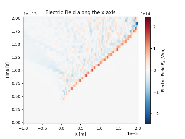
On top of accessing variables you can plot these xarray.Dataset
using the built-in xarray.DataArray.plot() function (see
https://docs.xarray.dev/en/stable/user-guide/plotting.html) which is
a simple call to matplotlib. This also means that you can access
all the methods from matplotlib to manipulate your plot.
# This is discretized in both space and time
In [12]: ds["Electric_Field_Ex"].plot()
Out[12]: <matplotlib.collections.QuadMesh at 0x7de1b5690800>

In [13]: plt.title("Electric Field along the x-axis")
Out[13]: Text(0.5, 1.0, 'Electric Field along the x-axis')
After having loaded in a series of datasets we can select a
simulation file by calling the xarray.Dataset.isel() function where we pass in
the parameter of time=0 where 0 can be a number between 0
and the total number of simulation files.
We can also use the xarray.Dataset.sel() function if we know the exact
simulation time we want to select. There must be a corresponding
dataset with this time for it work correctly.
In [14]: print(f"There are a total of {ds["time"].size} time steps. (This is the same as the number of SDF files in the folder)")
There are a total of 41 time steps. (This is the same as the number of SDF files in the folder)
In [15]: print("The time steps are: ")
The time steps are:
In [16]: print(ds["time"].values)
[2.60596949e-17 5.00346143e-15 1.00069229e-14 1.50103843e-14
2.00138457e-14 2.50173071e-14 3.00207686e-14 3.50242300e-14
4.00276914e-14 4.50311529e-14 5.00346143e-14 5.50380757e-14
6.00415371e-14 6.50449986e-14 7.00484600e-14 7.50519214e-14
8.00032635e-14 8.50067249e-14 9.00101863e-14 9.50136477e-14
1.00017109e-13 1.05020571e-13 1.10024032e-13 1.15027493e-13
1.20030955e-13 1.25034416e-13 1.30037878e-13 1.35041339e-13
1.40044801e-13 1.45048262e-13 1.50051723e-13 1.55003065e-13
1.60006527e-13 1.65009988e-13 1.70013450e-13 1.75016911e-13
1.80020373e-13 1.85023834e-13 1.90027295e-13 1.95030757e-13
2.00034218e-13]
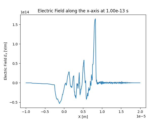
# The time at the 20th simulation step
In [17]: sim_time = ds['time'].isel(time=20).values
In [18]: print(f"The time at the 20th simulation step is {sim_time:.2e} s")
The time at the 20th simulation step is 1.00e-13 s
# We can plot the time using either the isel or sel method passing in either the index or the value of the time
In [19]: ds["Electric_Field_Ex"].isel(time=20).plot()
Out[19]: [<matplotlib.lines.Line2D at 0x7de1b6947260>]
# ds["Electric_Field_Ex"].sel(time=sim_time).plot()
In [20]: plt.title(f"Electric Field along the x-axis at {sim_time:.2e} s")
Out[20]: Text(0.5, 1.0, 'Electric Field along the x-axis at 1.00e-13 s')
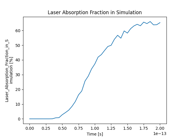
Manipulating Data#
These datasets can also be easily manipulated the same way as you
would with numpy arrays
In [21]: ds["Laser_Absorption_Fraction_in_Simulation"] = (ds["Total_Particle_Energy_in_Simulation"] / ds["Absorption_Total_Laser_Energy_Injected"]) * 100

# We can also manipulate the units and other attributes
In [22]: ds["Laser_Absorption_Fraction_in_Simulation"].attrs["units"] = "%"

In [23]: ds["Laser_Absorption_Fraction_in_Simulation"].plot()
Out[23]: [<matplotlib.lines.Line2D at 0x7de1b5b540e0>]

In [24]: plt.title("Laser Absorption Fraction in Simulation")
Out[24]: Text(0.5, 1.0, 'Laser Absorption Fraction in Simulation')
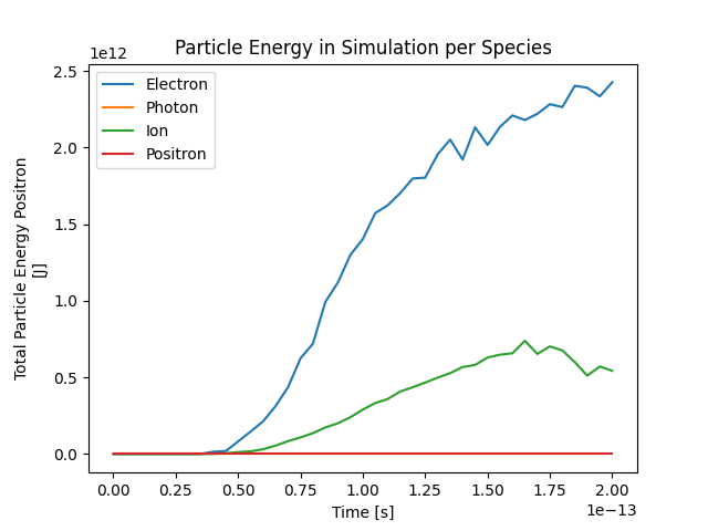
You can also call the plot() function on several variables with
labels by delaying the call to plt.show()
In [25]: print(f"The total laser energy injected into the simulation is {ds["Absorption_Total_Laser_Energy_Injected"].max().values:.1e} J")
The total laser energy injected into the simulation is 4.5e+12 J

In [26]: print(f"The total particle energy absorbed by the simulation is {ds["Total_Particle_Energy_in_Simulation"].max().values:.1e} J")
The total particle energy absorbed by the simulation is 3.0e+12 J

In [27]: print(f"The laser absorption fraction in the simulation is {ds["Laser_Absorption_Fraction_in_Simulation"].max().values:.1f} %")
The laser absorption fraction in the simulation is 66.0 %

In [28]: ds["Total_Particle_Energy_Electron"].plot(label="Electron")
Out[28]: [<matplotlib.lines.Line2D at 0x7de1b6737f80>]

In [29]: ds["Total_Particle_Energy_Photon"].plot(label="Photon")
Out[29]: [<matplotlib.lines.Line2D at 0x7de1b67347d0>]

In [30]: ds["Total_Particle_Energy_Ion"].plot(label="Ion")
Out[30]: [<matplotlib.lines.Line2D at 0x7de1b67371d0>]

In [31]: ds["Total_Particle_Energy_Positron"].plot(label="Positron")
Out[31]: [<matplotlib.lines.Line2D at 0x7de1b6736390>]

In [32]: plt.legend()
Out[32]: <matplotlib.legend.Legend at 0x7de1b666b2f0>

In [33]: plt.title("Particle Energy in Simulation per Species")
Out[33]: Text(0.5, 1.0, 'Particle Energy in Simulation per Species')