Key Functionality#

import xarray as xr
import sdf_xarray as sdfxr
import matplotlib.pyplot as plt
%matplotlib inline

Loading SDF files#

Loading raw files#

If you wish to load data directly from the SDF.C library and ignore the xarray interface layer.

raw_ds = sdfxr.SDFFile("tutorial_dataset_1d/0010.sdf")
raw_ds.variables.keys()

dict_keys(['Wall-time', 'Electric Field/Ex', 'Electric Field/Ey', 'Magnetic Field/Bz', 'Total Particle Energy/Electron', 'Total Particle Energy/Ion', 'Total Particle Energy in Simulation', 'Total Field Energy in Simulation', 'Derived/Number_Density/Electron', 'Derived/Number_Density/Ion', 'Derived/Temperature/Electron', 'Derived/Temperature/Ion', 'dist_fn/px_py/Electron', 'Electron_Probe/Px', 'Electron_Probe/Py', 'Electron_Probe/Pz', 'Electron_Probe/weight', 'Absorption/Total Laser Energy Injected', 'Absorption/Fraction of Laser Energy Absorbed', 'CPUs/Original rank', 'CPUs/Current rank'])

Loading multiple files#

Multiple files can be loaded using one of two methods. The first of which is by using the sdf_xarray.open_mfdataset.

Tip

If your simulation includes multiple output blocks that specify different variables for output at various time steps, variables not present at a specific step will default to a nan value. To remove these nan values we suggest using the xarray.DataArray.dropna function or following our implmentation in Loading sparse data.

sdfxr.open_mfdataset("tutorial_dataset_1d/*.sdf")

<xarray.Dataset> Size: 14MB
Dimensions:                                       (time: 41, X_Grid_mid: 200,
                                                   Px_px_py_Electron: 200,
                                                   Py_px_py_Electron: 200,
                                                   X_Grid: 201,
                                                   Px_px_py_Electron_mid: 199,
                                                   Py_px_py_Electron_mid: 199)
Coordinates:
  * time                                          (time) float64 328B 1.334e-...
  * X_Grid_mid                                    (X_Grid_mid) float64 2kB -4...
  * Px_px_py_Electron                             (Px_px_py_Electron) float64 2kB ...
  * Py_px_py_Electron                             (Py_px_py_Electron) float64 2kB ...
  * X_Grid                                        (X_Grid) float64 2kB -5e-06...
  * Px_px_py_Electron_mid                         (Px_px_py_Electron_mid) float64 2kB ...
  * Py_px_py_Electron_mid                         (Py_px_py_Electron_mid) float64 2kB ...
Data variables: (12/15)
    Wall_time                                     (time) float64 328B 0.00419...
    Electric_Field_Ex                             (time, X_Grid_mid) float64 66kB dask.array<chunksize=(1, 200), meta=np.ndarray>
    Electric_Field_Ey                             (time, X_Grid_mid) float64 66kB dask.array<chunksize=(1, 200), meta=np.ndarray>
    Magnetic_Field_Bz                             (time, X_Grid_mid) float64 66kB dask.array<chunksize=(1, 200), meta=np.ndarray>
    Total_Particle_Energy_Electron                (time) float64 328B 3.639e+...
    Total_Particle_Energy_Ion                     (time) float64 328B 3.57e+0...
    ...                                            ...
    Derived_Number_Density_Ion                    (time, X_Grid_mid) float64 66kB dask.array<chunksize=(1, 200), meta=np.ndarray>
    Derived_Temperature_Electron                  (time, X_Grid_mid) float64 66kB dask.array<chunksize=(1, 200), meta=np.ndarray>
    Derived_Temperature_Ion                       (time, X_Grid_mid) float64 66kB dask.array<chunksize=(1, 200), meta=np.ndarray>
    dist_fn_px_py_Electron                        (time, Px_px_py_Electron, Py_px_py_Electron) float64 13MB dask.array<chunksize=(1, 200, 200), meta=np.ndarray>
    Absorption_Total_Laser_Energy_Injected        (time) float64 328B 1.416e+...
    Absorption_Fraction_of_Laser_Energy_Absorbed  (time) float64 328B 0.0 ......
Attributes: (12/22)
    filename:         /home/docs/checkouts/readthedocs.org/user_builds/sdf-xa...
    file_version:     1
    file_revision:    4
    code_name:        Epoch1d
    step:             0
    time:             1.3342563807926084e-16
    ...               ...
    compile_flags:    unknown
    defines:          50364612
    compile_date:     Wed May 14 13:13:41 2025
    run_date:         Wed Nov 12 12:44:42 2025
    io_date:          Wed Nov 12 12:44:42 2025
    deck:             {'constant': {'I_peak': 1e+24, 'lambda_L': 1e-06, 't_fw...

Alternatively, files can be loaded using xarray.open_mfdataset however when loading in all the files we have do some processing of the data so that we can correctly align it along the time dimension; This is done via the preprocess parameter utilising the sdf_xarray.SDFPreprocess function.

xr.open_mfdataset(
   "tutorial_dataset_1d/*.sdf",
   join="outer",
   compat="no_conflicts",
   preprocess=sdfxr.SDFPreprocess()
)

<xarray.Dataset> Size: 14MB
Dimensions:                                       (time: 41, X_Grid_mid: 200,
                                                   Px_px_py_Electron: 200,
                                                   Py_px_py_Electron: 200,
                                                   X_Grid: 201,
                                                   Px_px_py_Electron_mid: 199,
                                                   Py_px_py_Electron_mid: 199)
Coordinates:
  * time                                          (time) float64 328B 1.334e-...
  * X_Grid_mid                                    (X_Grid_mid) float64 2kB -4...
  * Px_px_py_Electron                             (Px_px_py_Electron) float64 2kB ...
  * Py_px_py_Electron                             (Py_px_py_Electron) float64 2kB ...
  * X_Grid                                        (X_Grid) float64 2kB -5e-06...
  * Px_px_py_Electron_mid                         (Px_px_py_Electron_mid) float64 2kB ...
  * Py_px_py_Electron_mid                         (Py_px_py_Electron_mid) float64 2kB ...
Data variables: (12/15)
    Wall_time                                     (time) float64 328B 0.00419...
    Electric_Field_Ex                             (time, X_Grid_mid) float64 66kB dask.array<chunksize=(1, 200), meta=np.ndarray>
    Electric_Field_Ey                             (time, X_Grid_mid) float64 66kB dask.array<chunksize=(1, 200), meta=np.ndarray>
    Magnetic_Field_Bz                             (time, X_Grid_mid) float64 66kB dask.array<chunksize=(1, 200), meta=np.ndarray>
    Total_Particle_Energy_Electron                (time) float64 328B 3.639e+...
    Total_Particle_Energy_Ion                     (time) float64 328B 3.57e+0...
    ...                                            ...
    Derived_Number_Density_Ion                    (time, X_Grid_mid) float64 66kB dask.array<chunksize=(1, 200), meta=np.ndarray>
    Derived_Temperature_Electron                  (time, X_Grid_mid) float64 66kB dask.array<chunksize=(1, 200), meta=np.ndarray>
    Derived_Temperature_Ion                       (time, X_Grid_mid) float64 66kB dask.array<chunksize=(1, 200), meta=np.ndarray>
    dist_fn_px_py_Electron                        (time, Px_px_py_Electron, Py_px_py_Electron) float64 13MB dask.array<chunksize=(1, 200, 200), meta=np.ndarray>
    Absorption_Total_Laser_Energy_Injected        (time) float64 328B 1.416e+...
    Absorption_Fraction_of_Laser_Energy_Absorbed  (time) float64 328B 0.0 ......
Attributes: (12/22)
    filename:         /home/docs/checkouts/readthedocs.org/user_builds/sdf-xa...
    file_version:     1
    file_revision:    4
    code_name:        Epoch1d
    step:             0
    time:             1.3342563807926084e-16
    ...               ...
    compile_flags:    unknown
    defines:          50364612
    compile_date:     Wed May 14 13:13:41 2025
    run_date:         Wed Nov 12 12:44:42 2025
    io_date:          Wed Nov 12 12:44:42 2025
    deck:             {'constant': {'I_peak': 1e+24, 'lambda_L': 1e-06, 't_fw...

You can also load the data in as a xarray.DataTree, which organises the data hierarchically into groups (for example grouping related quantities such as the individual components of the electric and magnetic fields) while keeping each item as a xarray.Dataset.

sdfxr.open_mfdatatree("tutorial_dataset_1d/*.sdf")

<xarray.DataTree>
Group: /
│   Dimensions:                              (time: 41)
│   Coordinates:
│     * time                                 (time) float64 328B 1.334e-16 ... 2....
│   Data variables:
│       Wall-time                            (time) float64 328B 0.004197 ... 1.028
│       Total_Particle_Energy_in_Simulation  (time) float64 328B 7.209e+06 ... 1....
│       Total_Field_Energy_in_Simulation     (time) float64 328B 0.0 ... 1.25e+09
│   Attributes: (12/22)
│       filename:         /home/docs/checkouts/readthedocs.org/user_builds/sdf-xa...
│       file_version:     1
│       file_revision:    4
│       code_name:        Epoch1d
│       step:             0
│       time:             1.3342563807926084e-16
│       ...               ...
│       compile_flags:    unknown
│       defines:          50364612
│       compile_date:     Wed May 14 13:13:41 2025
│       run_date:         Wed Nov 12 12:44:42 2025
│       io_date:          Wed Nov 12 12:44:42 2025
│       deck:             {'constant': {'I_peak': 1e+24, 'lambda_L': 1e-06, 't_fw...
├── Group: /Electric_Field
│       Dimensions:     (time: 41, X_Grid_mid: 200)
│       Coordinates:
│         * X_Grid_mid  (X_Grid_mid) float64 2kB -4.95e-06 -4.85e-06 ... 1.495e-05
│       Data variables:
│           Ex          (time, X_Grid_mid) float64 66kB dask.array<chunksize=(1, 200), meta=np.ndarray>
│           Ey          (time, X_Grid_mid) float64 66kB dask.array<chunksize=(1, 200), meta=np.ndarray>
├── Group: /Magnetic_Field
│       Dimensions:     (time: 41, X_Grid_mid: 200)
│       Coordinates:
│         * X_Grid_mid  (X_Grid_mid) float64 2kB -4.95e-06 -4.85e-06 ... 1.495e-05
│       Data variables:
│           Bz          (time, X_Grid_mid) float64 66kB dask.array<chunksize=(1, 200), meta=np.ndarray>
├── Group: /Total_Particle_Energy
│       Dimensions:   (time: 41)
│       Data variables:
│           Electron  (time) float64 328B 3.639e+06 3.601e+06 ... 1.083e+10 1.07e+10
│           Ion       (time) float64 328B 3.57e+06 3.57e+06 ... 1.301e+09 1.313e+09
├── Group: /Absorption
│       Dimensions:                            (time: 41)
│       Data variables:
│           Total_Laser_Energy_Injected        (time) float64 328B 1.416e+06 ... 1.70...
│           Fraction_of_Laser_Energy_Absorbed  (time) float64 328B 0.0 0.9661 ... 0.5871
├── Group: /Derived
│   ├── Group: /Derived/Number_Density
│   │       Dimensions:     (time: 41, X_Grid_mid: 200)
│   │       Coordinates:
│   │         * X_Grid_mid  (X_Grid_mid) float64 2kB -4.95e-06 -4.85e-06 ... 1.495e-05
│   │       Data variables:
│   │           Electron    (time, X_Grid_mid) float64 66kB dask.array<chunksize=(1, 200), meta=np.ndarray>
│   │           Ion         (time, X_Grid_mid) float64 66kB dask.array<chunksize=(1, 200), meta=np.ndarray>
│   └── Group: /Derived/Temperature
│           Dimensions:     (time: 41, X_Grid_mid: 200)
│           Coordinates:
│             * X_Grid_mid  (X_Grid_mid) float64 2kB -4.95e-06 -4.85e-06 ... 1.495e-05
│           Data variables:
│               Electron    (time, X_Grid_mid) float64 66kB dask.array<chunksize=(1, 200), meta=np.ndarray>
│               Ion         (time, X_Grid_mid) float64 66kB dask.array<chunksize=(1, 200), meta=np.ndarray>
└── Group: /dist_fn
    └── Group: /dist_fn/px_py
            Dimensions:            (time: 41, Px_px_py_Electron: 200, Py_px_py_Electron: 200)
            Coordinates:
              * Px_px_py_Electron  (Px_px_py_Electron) float64 2kB -1.492e-21 ... 1.492e-21
              * Py_px_py_Electron  (Py_px_py_Electron) float64 2kB -1.492e-21 ... 1.492e-21
            Data variables:
                Electron           (time, Px_px_py_Electron, Py_px_py_Electron) float64 13MB dask.array<chunksize=(1, 200, 200), meta=np.ndarray>

Loading sparse data#

When dealing with sparse data (where different variables are saved at different, non-overlapping time steps) you can optimize memory usage by loading the data with sdf_xarray.open_mfdataset using the parameter separate_times=True. This approach creates a distinct time dimension for each output block, avoiding the need for a single, large time dimension that would be filled with nan values. This significantly reduces memory consumption, though it requires more deliberate handling if you need to compare variables that exist on these different time coordinates.

sdfxr.open_mfdataset("tutorial_dataset_1d/*.sdf", separate_times=True)

<xarray.Dataset> Size: 14MB
Dimensions:                                       (time0: 41, X_Grid_mid: 200,
                                                   Px_px_py_Electron: 200,
                                                   Py_px_py_Electron: 200,
                                                   X_Grid: 201,
                                                   Px_px_py_Electron_mid: 199,
                                                   Py_px_py_Electron_mid: 199)
Coordinates:
  * time0                                         (time0) float64 328B 1.334e...
  * X_Grid_mid                                    (X_Grid_mid) float64 2kB -4...
  * Px_px_py_Electron                             (Px_px_py_Electron) float64 2kB ...
  * Py_px_py_Electron                             (Py_px_py_Electron) float64 2kB ...
  * X_Grid                                        (X_Grid) float64 2kB -5e-06...
  * Px_px_py_Electron_mid                         (Px_px_py_Electron_mid) float64 2kB ...
  * Py_px_py_Electron_mid                         (Py_px_py_Electron_mid) float64 2kB ...
Data variables: (12/15)
    Wall_time                                     (time0) float64 328B 0.0041...
    Electric_Field_Ex                             (time0, X_Grid_mid) float64 66kB dask.array<chunksize=(1, 200), meta=np.ndarray>
    Electric_Field_Ey                             (time0, X_Grid_mid) float64 66kB dask.array<chunksize=(1, 200), meta=np.ndarray>
    Magnetic_Field_Bz                             (time0, X_Grid_mid) float64 66kB dask.array<chunksize=(1, 200), meta=np.ndarray>
    Total_Particle_Energy_Electron                (time0) float64 328B 3.639e...
    Total_Particle_Energy_Ion                     (time0) float64 328B 3.57e+...
    ...                                            ...
    Derived_Number_Density_Ion                    (time0, X_Grid_mid) float64 66kB dask.array<chunksize=(1, 200), meta=np.ndarray>
    Derived_Temperature_Electron                  (time0, X_Grid_mid) float64 66kB dask.array<chunksize=(1, 200), meta=np.ndarray>
    Derived_Temperature_Ion                       (time0, X_Grid_mid) float64 66kB dask.array<chunksize=(1, 200), meta=np.ndarray>
    dist_fn_px_py_Electron                        (time0, Px_px_py_Electron, Py_px_py_Electron) float64 13MB dask.array<chunksize=(1, 200, 200), meta=np.ndarray>
    Absorption_Total_Laser_Energy_Injected        (time0) float64 328B 1.416e...
    Absorption_Fraction_of_Laser_Energy_Absorbed  (time0) float64 328B 0.0 .....
Attributes: (12/18)
    file_version:     1
    file_revision:    4
    code_name:        Epoch1d
    jobid1:           1762951482
    jobid2:           578
    code_io_version:  1
    ...               ...
    compile_machine:  uoy24x520
    compile_flags:    unknown
    defines:          50364612
    compile_date:     Wed May 14 13:13:41 2025
    run_date:         Wed Nov 12 12:44:42 2025
    deck:             {'constant': {'I_peak': 1e+24, 'lambda_L': 1e-06, 't_fw...

Loading particle data#

Warning

It is not recommended to use xarray.open_mfdataset or sdf_xarray.open_mfdataset to load particle data from multiple SDF outputs. The number of particles often varies between outputs, which can lead to inconsistent array shapes that these functions cannot handle. Instead, consider loading each file individually and then concatenating them manually.

Note

When loading multiple probes from a single SDF file, you must use the probe_names parameter to assign a unique name to each. For example, use probe_names=["Front_Electron_Probe", "Back_Electron_Probe"]. Failing to do so will result in dimension name conflicts.

By default, particle data isn’t kept as it takes up a lot of space. Pass keep_particles=True as a keyword argument to xarray.open_dataset (for single files) or xarray.open_mfdataset (for multiple files).

Loading specific variables#

When loading datasets containing several (>10) coordinates/dimensions using sdf_xarray.open_mfdataset, xarray may struggle to locate the necessary RAM to concatenate all of the data (as seen in Issue #57). In this instance, you can optimize memory usage by loading only the data you need using the keyword argument data_vars and passing one or more variables. This creates a dataset consisting only of the given variable(s) and the relevant coordinates/dimensions, significantly reducing memory consumption.

sdfxr.open_mfdataset("tutorial_dataset_1d/*.sdf", data_vars=["Electric_Field_Ex"])

<xarray.Dataset> Size: 68kB
Dimensions:            (time: 41, X_Grid_mid: 200)
Coordinates:
  * time               (time) float64 328B 1.334e-16 5.07e-15 ... 2.001e-13
  * X_Grid_mid         (X_Grid_mid) float64 2kB -4.95e-06 ... 1.495e-05
Data variables:
    Electric_Field_Ex  (time, X_Grid_mid) float64 66kB dask.array<chunksize=(1, 200), meta=np.ndarray>
Attributes: (12/22)
    filename:         /home/docs/checkouts/readthedocs.org/user_builds/sdf-xa...
    file_version:     1
    file_revision:    4
    code_name:        Epoch1d
    step:             0
    time:             1.3342563807926084e-16
    ...               ...
    compile_flags:    unknown
    defines:          50364612
    compile_date:     Wed May 14 13:13:41 2025
    run_date:         Wed Nov 12 12:44:42 2025
    io_date:          Wed Nov 12 12:44:42 2025
    deck:             {'constant': {'I_peak': 1e+24, 'lambda_L': 1e-06, 't_fw...

Loading the input.deck#

When loading SDF files, sdf_xarray will attempt to automatically load the input.deck file used to initialise the simulation from the same directory as the SDF file. If the file is not found, it will silently fail and continue loading the SDF file as normal. This file contains the initial simulation setup information which is not present in SDF outputs. By loading this file, you can access these parameters as part of your dataset’s metadata. To do this, use the deck_path parameter when loading an SDF file with sdf_xarray.open_dataset, xarray.open_dataset, sdf_xarray.open_datatree, xarray.open_datatree, sdf_xarray.open_mfdataset or sdf_xarray.open_mfdatatree.

There are a few ways you can load an input deck:

Default behaviour: The input deck is loaded from the same directory as the SDF file if it exists. If it does not exist, it will silently fail.
Relative path: (e.g. "template.deck") Searches for that specific filename within the same directory as the SDF file.
Absolute path: (e.g. "/path/to/input.deck") Uses the full, specified path to locate the file.

An example of loading a deck can be seen below

import json
from IPython.display import Code

ds = xr.open_dataset("tutorial_dataset_1d/0010.sdf")
# The results are accessible by calling
deck = ds.attrs["deck"]

# Some prettification to make it looks nice in jupyter notebooks
json_str = json.dumps(deck, indent=4)
Code(json_str, language='json')

{
    "constant": {
        "I_peak": 1e+24,
        "lambda_L": 1e-06,
        "t_fwhm_L": 1.6e-14,
        "n_elec": 1e+27,
        "density_profile": "if(x lt 0, 0, 1)",
        "mppc": 50,
        "min_den_fact": 0.0001,
        "t_w": "t_fwhm_L / (sqrt(2*loge(2)))",
        "t_hw01m": "t_w * sqrt(loge(10))"
    },
    "control": {
        "t_end": 2e-13,
        "nx": 200,
        "x_min": -5e-06,
        "x_max": 1.5e-05,
        "nparticles": "nint( x_max / (x_max - x_min) * nx * mppc)",
        "dt_multiplier": 0.8,
        "smooth_currents": true,
        "dlb_threshold": 0.8,
        "stdout_frequency": 100
    },
    "laser": {
        "boundary": "x_min",
        "intensity": "I_peak",
        "lambda": "lambda_L",
        "t_profile": "gauss(time, t_hw01m, t_w)",
        "phase": 0
    },
    "boundaries": {
        "bc_x_min_field": "simple_laser",
        "bc_x_max_field": "simple_outflow",
        "bc_x_min_particle": "reflect",
        "bc_x_max_particle": "reflect"
    },
    "species": {
        "Electron": {
            "name": "Electron",
            "frac": 0.5,
            "temp_ev": 1000.0,
            "number_density_min": "n_elec * min_den_fact",
            "number_density": "n_elec * density_profile",
            "identify": "electron"
        },
        "Ion": {
            "name": "Ion",
            "frac": 0.5,
            "temp": "temp_x(Electron)",
            "number_density_min": "n_elec * min_den_fact",
            "number_density": "n_elec * density_profile",
            "identify": "proton"
        }
    },
    "dist_fn": {
        "px_py": {
            "name": "px_py",
            "ndims": 2,
            "dumpmask": "always",
            "direction1": "dir_px",
            "direction2": "dir_py",
            "range1": [
                -1.5e-21,
                1.5e-21
            ],
            "range2": [
                -1.5e-21,
                1.5e-21
            ],
            "resolution1": 200,
            "resolution2": 200,
            "include_species": "Electron"
        }
    },
    "probe": {
        "Electron_Probe": {
            "name": "Electron_Probe",
            "point": 0,
            "normal": -1,
            "ek_min": 0,
            "ek_max": -1,
            "include_species": "Electron",
            "dumpmask": "always"
        }
    },
    "output_global": {
        "force_final_to_be_restartable": false
    },
    "output": {
        "normal": {
            "name": "normal",
            "dt_snapshot": 5e-15,
            "particles": "never",
            "px": "never",
            "py": "never",
            "pz": "never",
            "particle_weight": "never",
            "particle_probes": "always",
            "grid": "always",
            "ex": "always",
            "ey": "always",
            "bz": "always",
            "number_density": "always + species + no_sum",
            "temperature": "always + species + no_sum",
            "total_energy_sum": "always + species",
            "distribution_functions": "always",
            "absorption": "always"
        }
    }
}

Data interaction examples#

When loading in either a single dataset or a group of datasets you can access the following methods to explore the dataset:

ds.variables to list variables. (e.g. Electric Field, Magnetic Field, Particle Count)
ds.coords for accessing coordinates/dimensions. (e.g. x-axis, y-axis, time)
ds.attrs for metadata attached to the dataset. (e.g. filename, step, time)

It is important to note here that xarray lazily loads the data meaning that it only explicitly loads the results your currently looking at when you call .values

ds = sdfxr.open_mfdataset("tutorial_dataset_1d/*.sdf")

ds["Electric_Field_Ex"]

<xarray.DataArray 'Electric_Field_Ex' (time: 41, X_Grid_mid: 200)> Size: 66kB
dask.array<concatenate, shape=(41, 200), dtype=float64, chunksize=(1, 200), chunktype=numpy.ndarray>
Coordinates:
  * time        (time) float64 328B 1.334e-16 5.07e-15 ... 1.951e-13 2.001e-13
  * X_Grid_mid  (X_Grid_mid) float64 2kB -4.95e-06 -4.85e-06 ... 1.495e-05
Attributes:
    units:       V/m
    point_data:  False
    full_name:   Electric Field/Ex
    long_name:   Electric Field $E_x$

xarray.DataArray

'Electric_Field_Ex'

time: 41
X_Grid_mid: 200

dask.array<chunksize=(1, 200), meta=np.ndarray>

	Array	Chunk
Bytes	64.06 kiB	1.56 kiB
Shape	(41, 200)	(1, 200)
Dask graph	41 chunks in 124 graph layers
Data type	float64 numpy.ndarray

Coordinates: (2)

time

(time)

float64

1.334e-16 5.07e-15 ... 2.001e-13

units :: s
long_name :: Time
full_name :: time

array([1.334256e-16, 5.070174e-15, 1.014035e-14, 1.521052e-14, 2.001385e-14,
       2.508402e-14, 3.015419e-14, 3.522437e-14, 4.002769e-14, 4.509787e-14,
       5.016804e-14, 5.523821e-14, 6.004154e-14, 6.511171e-14, 7.018189e-14,
       7.525206e-14, 8.005538e-14, 8.512556e-14, 9.019573e-14, 9.526591e-14,
       1.000692e-13, 1.051394e-13, 1.102096e-13, 1.150129e-13, 1.200831e-13,
       1.251532e-13, 1.302234e-13, 1.350267e-13, 1.400969e-13, 1.451671e-13,
       1.502373e-13, 1.550406e-13, 1.601108e-13, 1.651809e-13, 1.702511e-13,
       1.750544e-13, 1.801246e-13, 1.851948e-13, 1.902650e-13, 1.950683e-13,
       2.001385e-13])

X_Grid_mid

(X_Grid_mid)

float64

-4.95e-06 -4.85e-06 ... 1.495e-05

long_name :: X
units :: m
point_data :: False
full_name :: Grid/Grid_mid

array([-4.950e-06, -4.850e-06, -4.750e-06, -4.650e-06, -4.550e-06, -4.450e-06,
       -4.350e-06, -4.250e-06, -4.150e-06, -4.050e-06, -3.950e-06, -3.850e-06,
       -3.750e-06, -3.650e-06, -3.550e-06, -3.450e-06, -3.350e-06, -3.250e-06,
       -3.150e-06, -3.050e-06, -2.950e-06, -2.850e-06, -2.750e-06, -2.650e-06,
       -2.550e-06, -2.450e-06, -2.350e-06, -2.250e-06, -2.150e-06, -2.050e-06,
       -1.950e-06, -1.850e-06, -1.750e-06, -1.650e-06, -1.550e-06, -1.450e-06,
       -1.350e-06, -1.250e-06, -1.150e-06, -1.050e-06, -9.500e-07, -8.500e-07,
       -7.500e-07, -6.500e-07, -5.500e-07, -4.500e-07, -3.500e-07, -2.500e-07,
       -1.500e-07, -5.000e-08,  5.000e-08,  1.500e-07,  2.500e-07,  3.500e-07,
        4.500e-07,  5.500e-07,  6.500e-07,  7.500e-07,  8.500e-07,  9.500e-07,
        1.050e-06,  1.150e-06,  1.250e-06,  1.350e-06,  1.450e-06,  1.550e-06,
        1.650e-06,  1.750e-06,  1.850e-06,  1.950e-06,  2.050e-06,  2.150e-06,
        2.250e-06,  2.350e-06,  2.450e-06,  2.550e-06,  2.650e-06,  2.750e-06,
        2.850e-06,  2.950e-06,  3.050e-06,  3.150e-06,  3.250e-06,  3.350e-06,
        3.450e-06,  3.550e-06,  3.650e-06,  3.750e-06,  3.850e-06,  3.950e-06,
        4.050e-06,  4.150e-06,  4.250e-06,  4.350e-06,  4.450e-06,  4.550e-06,
        4.650e-06,  4.750e-06,  4.850e-06,  4.950e-06,  5.050e-06,  5.150e-06,
        5.250e-06,  5.350e-06,  5.450e-06,  5.550e-06,  5.650e-06,  5.750e-06,
        5.850e-06,  5.950e-06,  6.050e-06,  6.150e-06,  6.250e-06,  6.350e-06,
        6.450e-06,  6.550e-06,  6.650e-06,  6.750e-06,  6.850e-06,  6.950e-06,
        7.050e-06,  7.150e-06,  7.250e-06,  7.350e-06,  7.450e-06,  7.550e-06,
        7.650e-06,  7.750e-06,  7.850e-06,  7.950e-06,  8.050e-06,  8.150e-06,
        8.250e-06,  8.350e-06,  8.450e-06,  8.550e-06,  8.650e-06,  8.750e-06,
        8.850e-06,  8.950e-06,  9.050e-06,  9.150e-06,  9.250e-06,  9.350e-06,
        9.450e-06,  9.550e-06,  9.650e-06,  9.750e-06,  9.850e-06,  9.950e-06,
        1.005e-05,  1.015e-05,  1.025e-05,  1.035e-05,  1.045e-05,  1.055e-05,
        1.065e-05,  1.075e-05,  1.085e-05,  1.095e-05,  1.105e-05,  1.115e-05,
        1.125e-05,  1.135e-05,  1.145e-05,  1.155e-05,  1.165e-05,  1.175e-05,
        1.185e-05,  1.195e-05,  1.205e-05,  1.215e-05,  1.225e-05,  1.235e-05,
        1.245e-05,  1.255e-05,  1.265e-05,  1.275e-05,  1.285e-05,  1.295e-05,
        1.305e-05,  1.315e-05,  1.325e-05,  1.335e-05,  1.345e-05,  1.355e-05,
        1.365e-05,  1.375e-05,  1.385e-05,  1.395e-05,  1.405e-05,  1.415e-05,
        1.425e-05,  1.435e-05,  1.445e-05,  1.455e-05,  1.465e-05,  1.475e-05,
        1.485e-05,  1.495e-05])

Attributes: (4)
units :
V/m
point_data :
False
full_name :
Electric Field/Ex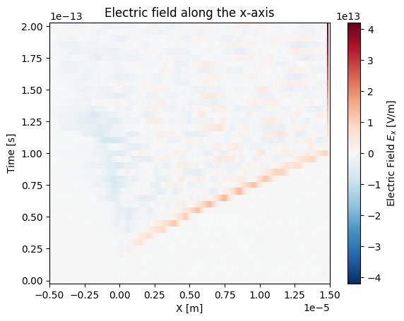
long_name :
Electric Field $E_x$

On top of accessing variables you can plot these xarray.Dataset using the built-in xarray.DataArray.plot function (see https://docs.xarray.dev/en/stable/user-guide/plotting.html) which is a simple call to matplotlib. This also means that you can access all the methods from matplotlib to manipulate your plot.

# This is discretized in both space and time
ds["Electric_Field_Ex"].plot()
plt.title("Electric field along the x-axis")
plt.show()

When loading a multi-file dataset using sdf_xarray.open_mfdataset, a time dimension is automatically added to the resulting xarray.Dataset. This dimension represents all the recorded simulation steps and allows for easy indexing. To quickly determine the number of time steps available, you can check the size of the time dimension.

# This corresponds to the number of individual SDF files loaded
print(f"There are a total of {ds['time'].size} time steps")

# You can look up the actual simulation time for any given index
sim_time = ds['time'].values[20]
print(f"The time at the 20th simulation step is {sim_time:.2e} s")

There are a total of 41 time steps
The time at the 20th simulation step is 1.00e-13 s

You can select and extract a single simulation snapshot using the integer index of the time step with the xarray.Dataset.isel function. This can be done by passsing the index to the time parameter (e.g., time=0 for the first snapshot).

# We can plot the variable at a given time index
ds["Electric_Field_Ex"].isel(time=20)

<xarray.DataArray 'Electric_Field_Ex' (X_Grid_mid: 200)> Size: 2kB
dask.array<getitem, shape=(200,), dtype=float64, chunksize=(200,), chunktype=numpy.ndarray>
Coordinates:
  * X_Grid_mid  (X_Grid_mid) float64 2kB -4.95e-06 -4.85e-06 ... 1.495e-05
    time        float64 8B 1.001e-13
Attributes:
    units:       V/m
    point_data:  False
    full_name:   Electric Field/Ex
    long_name:   Electric Field $E_x$

xarray.DataArray

'Electric_Field_Ex'

X_Grid_mid: 200

dask.array<chunksize=(200,), meta=np.ndarray>

	Array	Chunk
Bytes	1.56 kiB	1.56 kiB
Shape	(200,)	(200,)
Dask graph	1 chunks in 125 graph layers
Data type	float64 numpy.ndarray

Coordinates: (2)

X_Grid_mid

(X_Grid_mid)

float64

-4.95e-06 -4.85e-06 ... 1.495e-05

long_name :: X
units :: m
point_data :: False
full_name :: Grid/Grid_mid

array([-4.950e-06, -4.850e-06, -4.750e-06, -4.650e-06, -4.550e-06, -4.450e-06,
       -4.350e-06, -4.250e-06, -4.150e-06, -4.050e-06, -3.950e-06, -3.850e-06,
       -3.750e-06, -3.650e-06, -3.550e-06, -3.450e-06, -3.350e-06, -3.250e-06,
       -3.150e-06, -3.050e-06, -2.950e-06, -2.850e-06, -2.750e-06, -2.650e-06,
       -2.550e-06, -2.450e-06, -2.350e-06, -2.250e-06, -2.150e-06, -2.050e-06,
       -1.950e-06, -1.850e-06, -1.750e-06, -1.650e-06, -1.550e-06, -1.450e-06,
       -1.350e-06, -1.250e-06, -1.150e-06, -1.050e-06, -9.500e-07, -8.500e-07,
       -7.500e-07, -6.500e-07, -5.500e-07, -4.500e-07, -3.500e-07, -2.500e-07,
       -1.500e-07, -5.000e-08,  5.000e-08,  1.500e-07,  2.500e-07,  3.500e-07,
        4.500e-07,  5.500e-07,  6.500e-07,  7.500e-07,  8.500e-07,  9.500e-07,
        1.050e-06,  1.150e-06,  1.250e-06,  1.350e-06,  1.450e-06,  1.550e-06,
        1.650e-06,  1.750e-06,  1.850e-06,  1.950e-06,  2.050e-06,  2.150e-06,
        2.250e-06,  2.350e-06,  2.450e-06,  2.550e-06,  2.650e-06,  2.750e-06,
        2.850e-06,  2.950e-06,  3.050e-06,  3.150e-06,  3.250e-06,  3.350e-06,
        3.450e-06,  3.550e-06,  3.650e-06,  3.750e-06,  3.850e-06,  3.950e-06,
        4.050e-06,  4.150e-06,  4.250e-06,  4.350e-06,  4.450e-06,  4.550e-06,
        4.650e-06,  4.750e-06,  4.850e-06,  4.950e-06,  5.050e-06,  5.150e-06,
        5.250e-06,  5.350e-06,  5.450e-06,  5.550e-06,  5.650e-06,  5.750e-06,
        5.850e-06,  5.950e-06,  6.050e-06,  6.150e-06,  6.250e-06,  6.350e-06,
        6.450e-06,  6.550e-06,  6.650e-06,  6.750e-06,  6.850e-06,  6.950e-06,
        7.050e-06,  7.150e-06,  7.250e-06,  7.350e-06,  7.450e-06,  7.550e-06,
        7.650e-06,  7.750e-06,  7.850e-06,  7.950e-06,  8.050e-06,  8.150e-06,
        8.250e-06,  8.350e-06,  8.450e-06,  8.550e-06,  8.650e-06,  8.750e-06,
        8.850e-06,  8.950e-06,  9.050e-06,  9.150e-06,  9.250e-06,  9.350e-06,
        9.450e-06,  9.550e-06,  9.650e-06,  9.750e-06,  9.850e-06,  9.950e-06,
        1.005e-05,  1.015e-05,  1.025e-05,  1.035e-05,  1.045e-05,  1.055e-05,
        1.065e-05,  1.075e-05,  1.085e-05,  1.095e-05,  1.105e-05,  1.115e-05,
        1.125e-05,  1.135e-05,  1.145e-05,  1.155e-05,  1.165e-05,  1.175e-05,
        1.185e-05,  1.195e-05,  1.205e-05,  1.215e-05,  1.225e-05,  1.235e-05,
        1.245e-05,  1.255e-05,  1.265e-05,  1.275e-05,  1.285e-05,  1.295e-05,
        1.305e-05,  1.315e-05,  1.325e-05,  1.335e-05,  1.345e-05,  1.355e-05,
        1.365e-05,  1.375e-05,  1.385e-05,  1.395e-05,  1.405e-05,  1.415e-05,
        1.425e-05,  1.435e-05,  1.445e-05,  1.455e-05,  1.465e-05,  1.475e-05,
        1.485e-05,  1.495e-05])

time
()
float64
1.001e-13
units :
s
long_name :
Time
full_name :
time
```
array(1.00069229e-13)
```

Attributes: (4)
units :
V/m
point_data :
False
full_name :
Electric Field/Ex
long_name :
Electric Field $E_x$

We can also use the xarray.Dataset.sel function if you wish to pass a value intead of an index.

Tip

If you know roughly what time you wish to select but not the exact value you can use the parameter method="nearest".

ds["Electric_Field_Ex"].sel(time=sim_time)

<xarray.DataArray 'Electric_Field_Ex' (X_Grid_mid: 200)> Size: 2kB
dask.array<getitem, shape=(200,), dtype=float64, chunksize=(200,), chunktype=numpy.ndarray>
Coordinates:
  * X_Grid_mid  (X_Grid_mid) float64 2kB -4.95e-06 -4.85e-06 ... 1.495e-05
    time        float64 8B 1.001e-13
Attributes:
    units:       V/m
    point_data:  False
    full_name:   Electric Field/Ex
    long_name:   Electric Field $E_x$

xarray.DataArray

'Electric_Field_Ex'

X_Grid_mid: 200

dask.array<chunksize=(200,), meta=np.ndarray>

	Array	Chunk
Bytes	1.56 kiB	1.56 kiB
Shape	(200,)	(200,)
Dask graph	1 chunks in 125 graph layers
Data type	float64 numpy.ndarray

Coordinates: (2)

X_Grid_mid

(X_Grid_mid)

float64

-4.95e-06 -4.85e-06 ... 1.495e-05

long_name :: X
units :: m
point_data :: False
full_name :: Grid/Grid_mid

array([-4.950e-06, -4.850e-06, -4.750e-06, -4.650e-06, -4.550e-06, -4.450e-06,
       -4.350e-06, -4.250e-06, -4.150e-06, -4.050e-06, -3.950e-06, -3.850e-06,
       -3.750e-06, -3.650e-06, -3.550e-06, -3.450e-06, -3.350e-06, -3.250e-06,
       -3.150e-06, -3.050e-06, -2.950e-06, -2.850e-06, -2.750e-06, -2.650e-06,
       -2.550e-06, -2.450e-06, -2.350e-06, -2.250e-06, -2.150e-06, -2.050e-06,
       -1.950e-06, -1.850e-06, -1.750e-06, -1.650e-06, -1.550e-06, -1.450e-06,
       -1.350e-06, -1.250e-06, -1.150e-06, -1.050e-06, -9.500e-07, -8.500e-07,
       -7.500e-07, -6.500e-07, -5.500e-07, -4.500e-07, -3.500e-07, -2.500e-07,
       -1.500e-07, -5.000e-08,  5.000e-08,  1.500e-07,  2.500e-07,  3.500e-07,
        4.500e-07,  5.500e-07,  6.500e-07,  7.500e-07,  8.500e-07,  9.500e-07,
        1.050e-06,  1.150e-06,  1.250e-06,  1.350e-06,  1.450e-06,  1.550e-06,
        1.650e-06,  1.750e-06,  1.850e-06,  1.950e-06,  2.050e-06,  2.150e-06,
        2.250e-06,  2.350e-06,  2.450e-06,  2.550e-06,  2.650e-06,  2.750e-06,
        2.850e-06,  2.950e-06,  3.050e-06,  3.150e-06,  3.250e-06,  3.350e-06,
        3.450e-06,  3.550e-06,  3.650e-06,  3.750e-06,  3.850e-06,  3.950e-06,
        4.050e-06,  4.150e-06,  4.250e-06,  4.350e-06,  4.450e-06,  4.550e-06,
        4.650e-06,  4.750e-06,  4.850e-06,  4.950e-06,  5.050e-06,  5.150e-06,
        5.250e-06,  5.350e-06,  5.450e-06,  5.550e-06,  5.650e-06,  5.750e-06,
        5.850e-06,  5.950e-06,  6.050e-06,  6.150e-06,  6.250e-06,  6.350e-06,
        6.450e-06,  6.550e-06,  6.650e-06,  6.750e-06,  6.850e-06,  6.950e-06,
        7.050e-06,  7.150e-06,  7.250e-06,  7.350e-06,  7.450e-06,  7.550e-06,
        7.650e-06,  7.750e-06,  7.850e-06,  7.950e-06,  8.050e-06,  8.150e-06,
        8.250e-06,  8.350e-06,  8.450e-06,  8.550e-06,  8.650e-06,  8.750e-06,
        8.850e-06,  8.950e-06,  9.050e-06,  9.150e-06,  9.250e-06,  9.350e-06,
        9.450e-06,  9.550e-06,  9.650e-06,  9.750e-06,  9.850e-06,  9.950e-06,
        1.005e-05,  1.015e-05,  1.025e-05,  1.035e-05,  1.045e-05,  1.055e-05,
        1.065e-05,  1.075e-05,  1.085e-05,  1.095e-05,  1.105e-05,  1.115e-05,
        1.125e-05,  1.135e-05,  1.145e-05,  1.155e-05,  1.165e-05,  1.175e-05,
        1.185e-05,  1.195e-05,  1.205e-05,  1.215e-05,  1.225e-05,  1.235e-05,
        1.245e-05,  1.255e-05,  1.265e-05,  1.275e-05,  1.285e-05,  1.295e-05,
        1.305e-05,  1.315e-05,  1.325e-05,  1.335e-05,  1.345e-05,  1.355e-05,
        1.365e-05,  1.375e-05,  1.385e-05,  1.395e-05,  1.405e-05,  1.415e-05,
        1.425e-05,  1.435e-05,  1.445e-05,  1.455e-05,  1.465e-05,  1.475e-05,
        1.485e-05,  1.495e-05])

time
()
float64
1.001e-13
units :
s
long_name :
Time
full_name :
time
```
array(1.00069229e-13)
```

Attributes: (4)
units :
V/m
point_data :
False
full_name :
Electric Field/Ex
long_name :
Electric Field $E_x$

Visualisation on HPCs#

In many cases you will be running EPOCH simulations via a HPC cluster and your subsequent SDF files will probably be rather large and cumbersome to interact with via traditional Jupyter notebooks. In some cases your HPC may outright block the use of Jupyter notebooks entirely. To circumvent this issue you can use a Terminal User Interface (TUI) which renders the contents of SDF files directly in a Terminal and allows for you to do some simple data analysis and visualisation. To do this we shall leverage the xr-tui package which can be installed to either a venv or globally using:

pip install xr-tui sdf-xarray

or if you are using uv

uv tool install xr-tui --with sdf-xarray

Once installed you can visualise SDF files by simply writing in the command line

xr path/to/simulation/0000.sdf
# OR
xr path/to/simulation/*.sdf

Below is an example gif of how this interfacing looks as seen on xr-tui README.md:

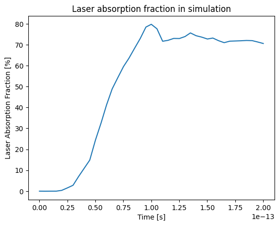
Manipulating data#

These datasets can also be easily manipulated the same way as you would with numpy arrays.

ds["Laser_Absorption_Fraction_in_Simulation"] = (
   (ds["Total_Particle_Energy_in_Simulation"] - ds["Total_Particle_Energy_in_Simulation"][0])
   / ds["Absorption_Total_Laser_Energy_Injected"]
) * 100

# We can also manipulate the units and other attributes
ds["Laser_Absorption_Fraction_in_Simulation"].attrs["units"] = "%"
ds["Laser_Absorption_Fraction_in_Simulation"].attrs["long_name"] = "Laser Absorption Fraction"

ds["Laser_Absorption_Fraction_in_Simulation"].plot()
plt.title("Laser absorption fraction in simulation")
plt.show()

You can also call the plot() function on several variables with labels by delaying the call to plt.show().

ds["Total_Particle_Energy_Electron"].plot(label="Electron")
ds["Total_Particle_Energy_Ion"].plot(label="Ion")
plt.title("Particle Energy in Simulation per Species")
plt.legend()
plt.show()

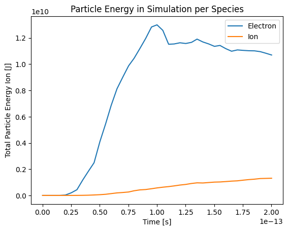
print(f"Total laser energy injected: {ds["Absorption_Total_Laser_Energy_Injected"][-1].values:.1e} J")
print(f"Total particle energy absorbed: {ds["Total_Particle_Energy_in_Simulation"][-1].values:.1e} J")
print(f"The laser absorption fraction: {ds["Laser_Absorption_Fraction_in_Simulation"][-1].values:.1f} %")

Total laser energy injected: 1.7e+10 J
Total particle energy absorbed: 1.2e+10 J
The laser absorption fraction: 70.6 %

Key Functionality

Contents

Key Functionality#

Loading SDF files#

Loading single files#

Loading raw files#

Loading multiple files#

Loading sparse data#

Loading particle data#

Loading specific variables#

Loading the input.deck#

Data interaction examples#

Visualisation on HPCs#

Manipulating data#